Plotting on original grid with cartopy
If you would like to try to repeat examples from this introduction, you can download FESOM2 data and mesh. The data are quite heavy, about 1.5Gb in bzip2 archive.
Link: https://swiftbrowser.dkrz.de/public/dkrz_c719fbc3-98ea-446c-8e01-356dac22ed90/PYFESOM2/
You have to download LCORE2.tar and core2.tar.bz2 archives and extract them.
Alternative would be to use very light weight mesh that comes with pyfesom2 in the tests/data/pi-grid/ and example data on this mesh in tests/data/pi-results.
Warning
Current version is still quite buggy, so don’t expect that thing are running ery smothly :) Please submit bug reports to:
Plotting variables located on nodes (vertices)
[1]:
import pyfesom2 as pf
import matplotlib.cm as cm
[2]:
mesh = pf.load_mesh('../../DATA/core2/')
/Users/nkolduno/PYTHON/DATA/core2/pickle_mesh_py3_fesom2
The usepickle == True)
The pickle file for FESOM2 exists.
The mesh will be loaded from /Users/nkolduno/PYTHON/DATA/core2/pickle_mesh_py3_fesom2
[3]:
data_path = '../../DATA/LCORE2/'
First load the data on the surface layer
[4]:
data = pf.get_data(data_path, "temp", [1948, 1949], mesh, how="mean", compute=True, depth=0)
Model depth: 0.0
Minimum input is mesh and data
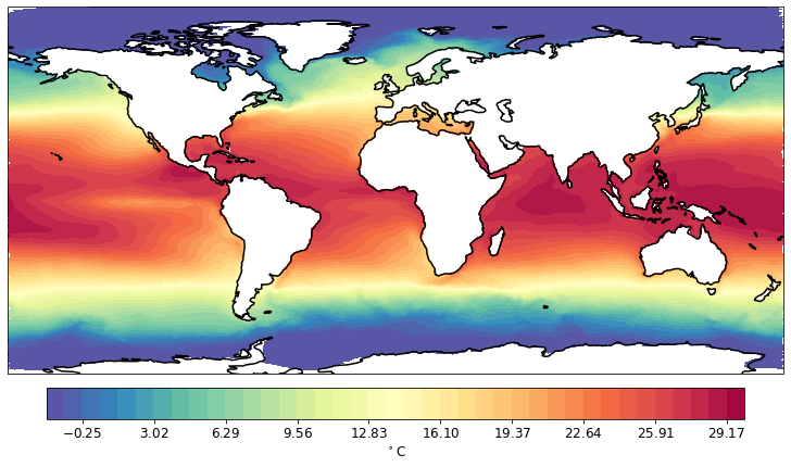
[5]:
%%time
pf.tplot(mesh, data)
CPU times: user 512 ms, sys: 19.6 ms, total: 531 ms
Wall time: 531 ms
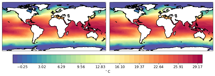
You can provide several data arrays as an input. You should specify rowcol variable then, to define how the output will be arranged.
[6]:
%%time
pf.tplot(mesh, [data, data], rowscol=(1,2))
CPU times: user 1.16 s, sys: 34.3 ms, total: 1.2 s
Wall time: 1.2 s
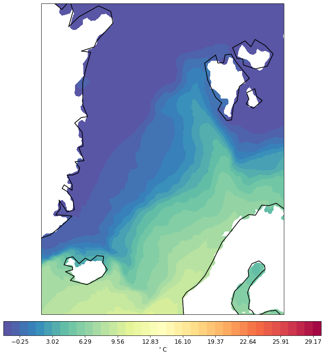
One can plot smallare resion by specifying the box.
TODO: - This does not work with standard pc at the moment (at least if the southern boundary is above the equator) - With merc projection only properly works untill 84N. Then show artefacts.
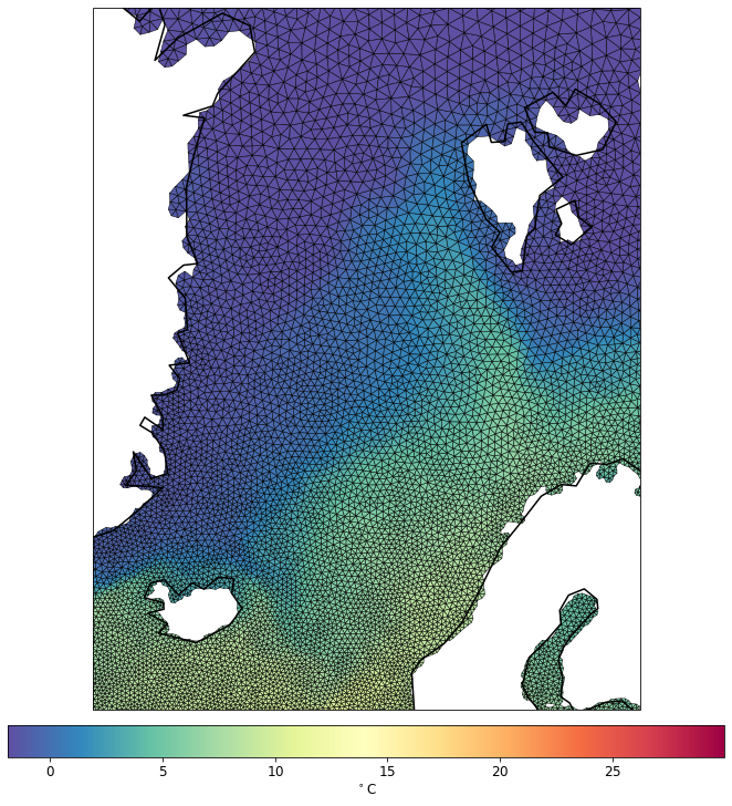
[7]:
%%time
pf.tplot(mesh, data, ptype='cf', box=[-30, 30, 60, 82], mapproj='merc')
CPU times: user 95.1 ms, sys: 4.51 ms, total: 99.6 ms
Wall time: 98 ms
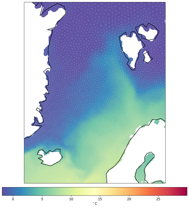
Instead of cf (tricontourf), one can change to the tri (tripcolor) plot.
TODO - This works with both merc and pc, and one can set the northern limit to 90.
[8]:
%%time
pf.tplot(mesh, data, ptype='tri', box=[-30, 30, 60, 82], mapproj='merc')
CPU times: user 5.03 s, sys: 25.5 ms, total: 5.06 s
Wall time: 4.79 s
To highlight the mesh structire more, you can change the lw parameter.
[9]:
%%time
pf.tplot(mesh, data, ptype='tri', box=[-30, 30, 60, 82], mapproj='merc', lw=0.5)
CPU times: user 4.98 s, sys: 33.1 ms, total: 5.01 s
Wall time: 4.78 s
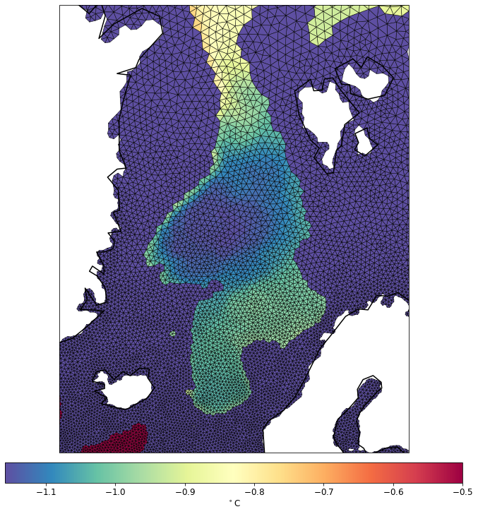
Let’s try different depth
[10]:
data = pf.get_data(data_path, "temp", [1948, 1949], mesh, how="mean", compute=True, depth=2000)
Model depth: 1920.0
TODO:
NaNs do not work for tri* functions somehow. We had to put the empty nodes to -99999.
For
tripcolorthis leads to filling of NaNs by the same color.One has to specify the range manually.
[11]:
%%time
pf.tplot(mesh, data, ptype='tri', box=[-30, 30, 60, 82], mapproj='merc', lw=0.5, levels=(-1.5, -0.5, 41))
minimum level changed to make cartopy happy
CPU times: user 4.97 s, sys: 52.2 ms, total: 5.02 s
Wall time: 4.8 s
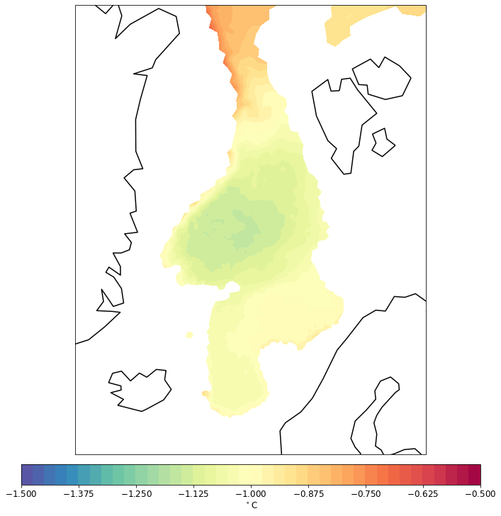
TODO:
For
cfthe NaNs (which are set to -9999) are not plotted, but one has to be again careful with specifying the range.
[12]:
%%time
pf.tplot(mesh, data, ptype='cf', box=[-30, 30, 60, 82], mapproj='merc', lw=0.5, levels=(-1.5, -0.5, 41))
CPU times: user 87.9 ms, sys: 5 ms, total: 92.9 ms
Wall time: 92.6 ms
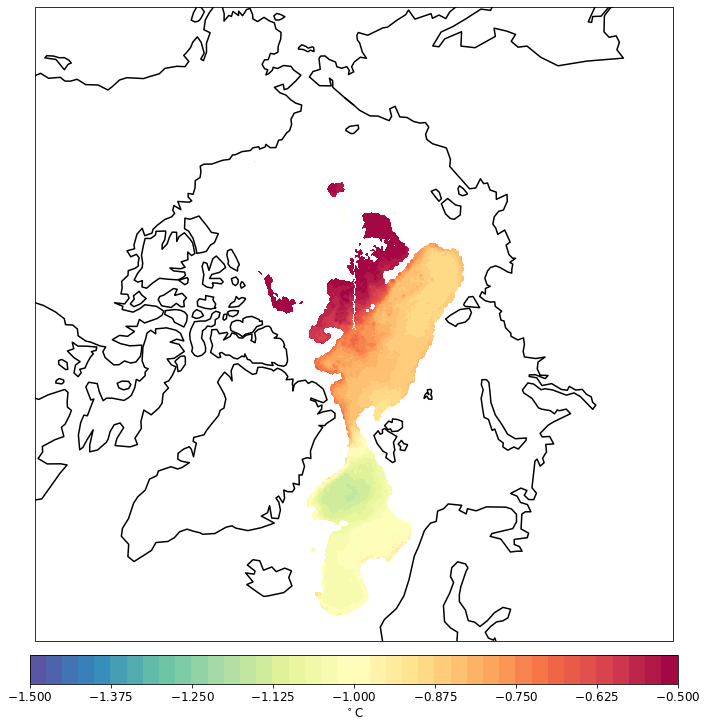
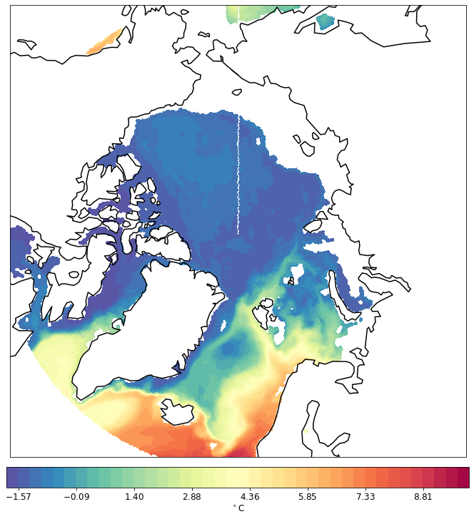
North polar stereo projection:
[13]:
%%time
pf.tplot(mesh, data, ptype='cf', box=[-180, 180, 60, 90], mapproj='np', lw=0.5, levels=(-1.5, -0.5, 41))
CPU times: user 178 ms, sys: 6.36 ms, total: 184 ms
Wall time: 184 ms
Also for the different depth.
TODO:
With Basemap it was possible to get rid of the line along 180 (by not using no_cyclic_elem). Now we have to live with it.
[14]:
data = pf.get_data(data_path, "temp", [1948, 1949], mesh, how="mean", compute=True, depth=100)
Model depth: 100.0
[15]:
%%time
pf.tplot(mesh, data, ptype='cf', box=[-180, 180, 60, 90], mapproj='np', lw=0.5, levels=(-2, 10, 41))
minimum level changed to make cartopy happy
CPU times: user 175 ms, sys: 5.21 ms, total: 180 ms
Wall time: 180 ms
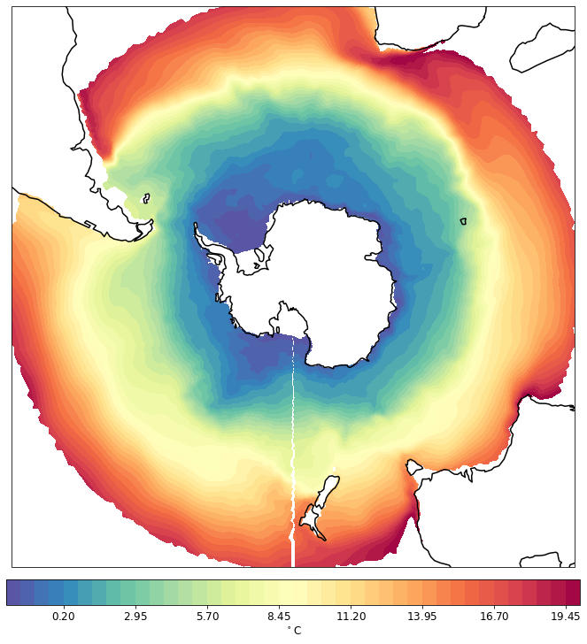
The South is working as well.
[16]:
%%time
pf.tplot(mesh, data, ptype='cf', box=[-180, 180, -90, -30], mapproj='sp', lw=0.5, levels=(-2, 20, 41))
CPU times: user 207 ms, sys: 5.36 ms, total: 212 ms
Wall time: 214 ms
Plotting on elements (faces)
[9]:
import pyfesom2 as pf
import matplotlib.cm as cm
[10]:
mesh = pf.load_mesh('../../DATA/core2/')
/Users/nkolduno/PYTHON/DATA/core2/pickle_mesh_py3_fesom2
The usepickle == True)
The pickle file for FESOM2 exists.
The mesh will be loaded from /Users/nkolduno/PYTHON/DATA/core2/pickle_mesh_py3_fesom2
[11]:
data_path = '../../DATA/LCORE2/'
[19]:
data = pf.get_data(data_path, "u", [1948, 1949], mesh, how="mean", compute=True, depth=0)
Model depth: 0.0
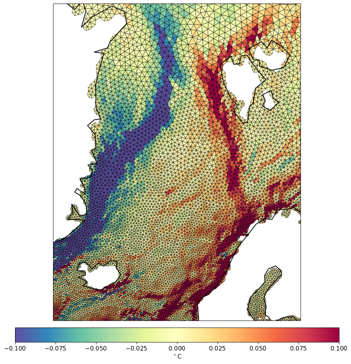
The only supported way to plot variables on elements (or faces) is to use ptype='tri'. The ploting for the whole globe is very slow, even if relatively small mesh is considered, so it is better to select smaller region.
[16]:
pf.tplot(mesh, data, ptype='tri',box=[-30, 30, 60, 82], mapproj='merc', lw=0.5, levels=(-0.1, 0.1, 41))
Example of np projection.
[17]:
pf.tplot(mesh, data, ptype='tri', box=[-180, 180, 70, 90], mapproj='np', lw=0.1,levels=(-0.1, 0.1, 41))
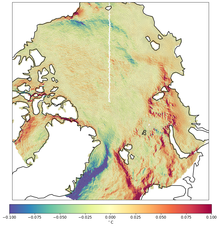
The blank line along 180 longitude is to avoid cartopy confusion with coordinates of elements that cross 180 line.
Plot at deeper layers
[21]:
data = pf.get_data(data_path, "u", [1948, 1949], mesh, how="mean", compute=True, depth=100)
pf.tplot(mesh, data, ptype='tri',box=[-100, -30, 20, 50], mapproj='merc', lw=0.5, levels=(-0.1, 0.1, 41))
Model depth: 100.0
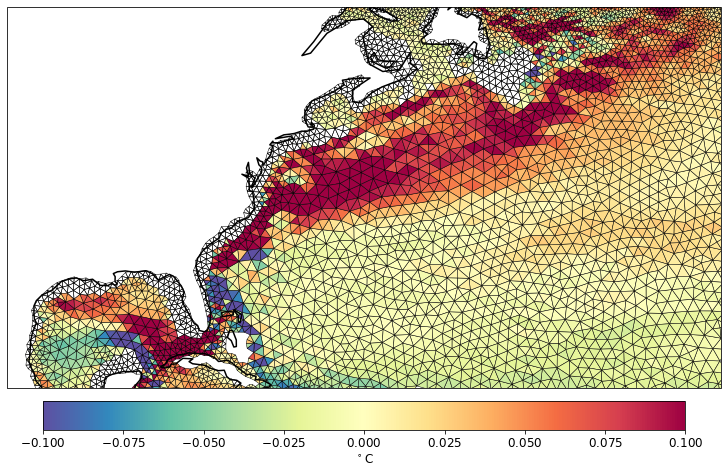
The surface mesh is still visible.
[ ]: