This page was generated from notebooks/accessor_selections.ipynb. Interactive online version: .

Data selection using pyfesom2’s xarray-accesor.

1. Introduction

A key feature of pyfesom2 is to facilitate spatial selections on its unstructured triangular grid, that is currently not supported by commonly used python libraries. Xarray provides a powerful label based selection on datasets and variables (dataarray). A similar interface is provided (with additional convinient features) for FESOM data through pyfesom2 accessor.

Xarray’s sel method takes dimension names of a dataset or datarray as arguments for selection. For rectiliner grids this provides easy interface to select arbitary points and rectangular regions (using slices) in latitudes and longitudes. In case of FESOM unstructured grid, latitudes, longitudes are not orthogonal to each other and are not part of dataset’s dimensions, insted they are coordinates of a common dimension nod2. This means the convinent spatial selection in xarray using latitude and longitude as indexers is not possible for FESOM data using regular sel(lat=..., lon=...) method. The dataset.pyfesom2.select(lat=..., lon=...) method of pyfesom2 provides alternative to do such selections on FESOM data. Being in a constrained data environment also allows us to more add convinient features such as selecting arbitarary polygons.

Because of differences in functionality, arguments, and to minimize confusion with xarray’s sel method, accessor’s selection methods are prefixed with select.

Load a tutorial dataset

While examples in this notebook use a remote version of FESOM2 data to make the notebook self-contained, one may choose to load a local raw-dataset or download a raw dataset as indicated in pyfesom2_overview.ipynb notebook.

To load such local data into a Xarray dataset (to be able to use the accessor) replace the cell below with:

from pyfesom2.datasets import open_dataset
mesh_path = "/Users/nkolduno/PYTHON/DATA/core2/"
data_path = "/Users/nkolduno/PYTHON/DATA/LCORE2/[temp,salt,a_ice,m_ice]*"
fesom_ds = open_dataset(data_path, mesh_path)

Of course one should replace paths to the ones located on your machine. The open_dataset function takes a parameter abg to support specifying rotations for a rotated grid, which might be needed if you work with legacy rotated meshes.

For other available remote datasets see remote datasets.ipynb notebook.

from pyfesom2.datasets import core
fesom_ds = core.load()
fesom_ds

<xarray.Dataset>
Dimensions:  (nelem: 243899, nod2: 126858, nz: 48, nz1: 47, three: 3, time: 144)
Coordinates:
  * time     (time) datetime64[ns] 1948-01-31T23:15:00 ... 1959-12-31T23:15:00
    lat      (nod2) float64 dask.array<chunksize=(31715,), meta=np.ndarray>
    lon      (nod2) float64 dask.array<chunksize=(31715,), meta=np.ndarray>
  * nz1      (nz1) float64 -2.5 -7.5 -15.0 ... -5.525e+03 -5.825e+03 -6.125e+03
    faces    (nelem, three) uint32 dask.array<chunksize=(60975, 2), meta=np.ndarray>
  * nz       (nz) float64 0.0 -5.0 -10.0 -20.0 ... -5.65e+03 -6e+03 -6.25e+03
Dimensions without coordinates: nelem, nod2, three
Data variables:
    temp     (time, nod2, nz1) float32 dask.array<chunksize=(1, 126858, 47), meta=np.ndarray>
    salt     (time, nod2, nz1) float32 dask.array<chunksize=(1, 126858, 47), meta=np.ndarray>
    a_ice    (time, nod2) float32 dask.array<chunksize=(1, 126858), meta=np.ndarray>
    m_ice    (time, nod2) float32 dask.array<chunksize=(1, 126858), meta=np.ndarray>
    ssh      (time, nod2) float32 dask.array<chunksize=(1, 126858), meta=np.ndarray>
    sst      (time, nod2) float32 dask.array<chunksize=(1, 126858), meta=np.ndarray>
Attributes:
    Dataset URL:  https://swiftbrowser.dkrz.de/public/dkrz_02942825-0cab-44f3...

2. Region selection

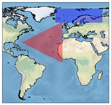
To select a rectangular region, bounds of bounding rectangle defined as (minlon, minlat, maxlon, maxlat) can be passed to region argument. To select arbitary polygons, Shapely’s Polygon object can be used as an argument to region. The region selection returns reindexed faces corresponding to selected points. This subsetted data may be saved to disk using regular xarray saving methods such as .to_netcdf(path_to_file.nc).

Select a rectangular region.

fesom_ds.pyfesom2.select(region=(-20, 60, 50, 80))

<xarray.Dataset>
Dimensions:  (nelem: 12737, nod2: 6699, nz: 48, nz1: 47, three: 3, time: 144)
Coordinates:
  * time     (time) datetime64[ns] 1948-01-31T23:15:00 ... 1959-12-31T23:15:00
    lat      (nod2) float64 dask.array<chunksize=(276,), meta=np.ndarray>
    lon      (nod2) float64 dask.array<chunksize=(276,), meta=np.ndarray>
  * nz1      (nz1) float64 -2.5 -7.5 -15.0 ... -5.525e+03 -5.825e+03 -6.125e+03
  * nz       (nz) float64 0.0 -5.0 -10.0 -20.0 ... -5.65e+03 -6e+03 -6.25e+03
    faces    (nelem, three) int64 3462 3464 66 59 3041 ... 2775 235 6698 2773
Dimensions without coordinates: nelem, nod2, three
Data variables:
    temp     (time, nod2, nz1) float32 dask.array<chunksize=(1, 6699, 47), meta=np.ndarray>
    salt     (time, nod2, nz1) float32 dask.array<chunksize=(1, 6699, 47), meta=np.ndarray>
    a_ice    (time, nod2) float32 dask.array<chunksize=(1, 6699), meta=np.ndarray>
    m_ice    (time, nod2) float32 dask.array<chunksize=(1, 6699), meta=np.ndarray>
    ssh      (time, nod2) float32 dask.array<chunksize=(1, 6699), meta=np.ndarray>
    sst      (time, nod2) float32 dask.array<chunksize=(1, 6699), meta=np.ndarray>
Attributes:
    Dataset URL:  https://swiftbrowser.dkrz.de/public/dkrz_02942825-0cab-44f3...

Select a triangular region defined by Shapely’s Polygon

from shapely.geometry import Polygon
polygon_region = Polygon([(-70, 30), (-10, 0), (-10, 60)])  # a triangle in atlantic
fesom_ds.pyfesom2.select(region=polygon_region)

<xarray.Dataset>
Dimensions:  (nelem: 7387, nod2: 3887, nz: 48, nz1: 47, three: 3, time: 144)
Coordinates:
  * time     (time) datetime64[ns] 1948-01-31T23:15:00 ... 1959-12-31T23:15:00
    lat      (nod2) float64 dask.array<chunksize=(711,), meta=np.ndarray>
    lon      (nod2) float64 dask.array<chunksize=(711,), meta=np.ndarray>
  * nz1      (nz1) float64 -2.5 -7.5 -15.0 ... -5.525e+03 -5.825e+03 -6.125e+03
  * nz       (nz) float64 0.0 -5.0 -10.0 -20.0 ... -5.65e+03 -6e+03 -6.25e+03
    faces    (nelem, three) int64 2088 2089 2090 3065 154 ... 3886 3013 617 3886
Dimensions without coordinates: nelem, nod2, three
Data variables:
    temp     (time, nod2, nz1) float32 dask.array<chunksize=(1, 3887, 47), meta=np.ndarray>
    salt     (time, nod2, nz1) float32 dask.array<chunksize=(1, 3887, 47), meta=np.ndarray>
    a_ice    (time, nod2) float32 dask.array<chunksize=(1, 3887), meta=np.ndarray>
    m_ice    (time, nod2) float32 dask.array<chunksize=(1, 3887), meta=np.ndarray>
    ssh      (time, nod2) float32 dask.array<chunksize=(1, 3887), meta=np.ndarray>
    sst      (time, nod2) float32 dask.array<chunksize=(1, 3887), meta=np.ndarray>
Attributes:
    Dataset URL:  https://swiftbrowser.dkrz.de/public/dkrz_02942825-0cab-44f3...

Other orthogonal dimensions to lat,lon such as time, nz1, may also be used similar to xarray’s sel method. Note that select method allows mixing of arrays for lat, lon as indexer and slices for other dimensions unlike Xarray for convinience.

fesom_ds.pyfesom2.select(region=polygon_region, time=slice('1950-01-01', '1950-05-02'))

<xarray.Dataset>
Dimensions:  (nelem: 7387, nod2: 3887, nz: 48, nz1: 47, three: 3, time: 4)
Coordinates:
  * time     (time) datetime64[ns] 1950-01-31T23:15:00 ... 1950-04-30T23:15:00
    lat      (nod2) float64 dask.array<chunksize=(711,), meta=np.ndarray>
    lon      (nod2) float64 dask.array<chunksize=(711,), meta=np.ndarray>
  * nz1      (nz1) float64 -2.5 -7.5 -15.0 ... -5.525e+03 -5.825e+03 -6.125e+03
  * nz       (nz) float64 0.0 -5.0 -10.0 -20.0 ... -5.65e+03 -6e+03 -6.25e+03
    faces    (nelem, three) int64 2088 2089 2090 3065 154 ... 3886 3013 617 3886
Dimensions without coordinates: nelem, nod2, three
Data variables:
    temp     (time, nod2, nz1) float32 dask.array<chunksize=(1, 3887, 47), meta=np.ndarray>
    salt     (time, nod2, nz1) float32 dask.array<chunksize=(1, 3887, 47), meta=np.ndarray>
    a_ice    (time, nod2) float32 dask.array<chunksize=(1, 3887), meta=np.ndarray>
    m_ice    (time, nod2) float32 dask.array<chunksize=(1, 3887), meta=np.ndarray>
    ssh      (time, nod2) float32 dask.array<chunksize=(1, 3887), meta=np.ndarray>
    sst      (time, nod2) float32 dask.array<chunksize=(1, 3887), meta=np.ndarray>
Attributes:
    Dataset URL:  https://swiftbrowser.dkrz.de/public/dkrz_02942825-0cab-44f3...

2. Point selection

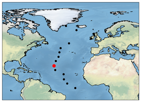
To select a data closest to a single point in latitude and longitude, select method can be supplied with lat, lon values as indexers such as:

fesom_ds.select(lon=-20, lat=10)

To select more points, that may define a transect in latitude and longitude, they can be provided as lat and lon arguments (and have to be of same size) containing sequence of values.

Note that point selection defaults to nearest neighbor selection on geocentric projection. This is equivalent to using tunnel distance for evaluating nearest neighbor.

Define points in latitude and longitude as numpy arrays and select closest data.

import numpy as np
sel_lats = np.linspace(-90,90,10)
sel_lons = np.linspace(-180,180,10)
fesom_ds.pyfesom2.select(lat= sel_lats, lon= sel_lons)

<xarray.Dataset>
Dimensions:  (nod2: 10, nz: 48, nz1: 47, time: 144)
Coordinates:
  * time     (time) datetime64[ns] 1948-01-31T23:15:00 ... 1959-12-31T23:15:00
    lat      (nod2) float64 dask.array<chunksize=(1,), meta=np.ndarray>
    lon      (nod2) float64 dask.array<chunksize=(1,), meta=np.ndarray>
  * nz1      (nz1) float64 -2.5 -7.5 -15.0 ... -5.525e+03 -5.825e+03 -6.125e+03
  * nz       (nz) float64 0.0 -5.0 -10.0 -20.0 ... -5.65e+03 -6e+03 -6.25e+03
Dimensions without coordinates: nod2
Data variables:
    temp     (time, nod2, nz1) float32 dask.array<chunksize=(1, 10, 47), meta=np.ndarray>
    salt     (time, nod2, nz1) float32 dask.array<chunksize=(1, 10, 47), meta=np.ndarray>
    a_ice    (time, nod2) float32 dask.array<chunksize=(1, 10), meta=np.ndarray>
    m_ice    (time, nod2) float32 dask.array<chunksize=(1, 10), meta=np.ndarray>
    ssh      (time, nod2) float32 dask.array<chunksize=(1, 10), meta=np.ndarray>
    sst      (time, nod2) float32 dask.array<chunksize=(1, 10), meta=np.ndarray>
Attributes:
    Dataset URL:  https://swiftbrowser.dkrz.de/public/dkrz_02942825-0cab-44f3...

Note that point selection does not return faces in coordinates, because faces contains indices and after selection they have no relavence, in future we may return lat and lon bnds

Additionally other dimensions can also be passed as indexers similar to Xarray’s sel method, in that case an orthogonal selection, ie., transect at selected times and levels is made.

fesom_ds.pyfesom2.select(lat= sel_lats, lon= sel_lons, nz1=slice(0, -1000))

<xarray.Dataset>
Dimensions:  (nod2: 10, nz: 48, nz1: 25, time: 144)
Coordinates:
  * time     (time) datetime64[ns] 1948-01-31T23:15:00 ... 1959-12-31T23:15:00
    lat      (nod2) float64 dask.array<chunksize=(1,), meta=np.ndarray>
    lon      (nod2) float64 dask.array<chunksize=(1,), meta=np.ndarray>
  * nz1      (nz1) float64 -2.5 -7.5 -15.0 -25.0 ... -630.0 -735.0 -850.0 -975.0
  * nz       (nz) float64 0.0 -5.0 -10.0 -20.0 ... -5.65e+03 -6e+03 -6.25e+03
Dimensions without coordinates: nod2
Data variables:
    temp     (time, nod2, nz1) float32 dask.array<chunksize=(1, 10, 25), meta=np.ndarray>
    salt     (time, nod2, nz1) float32 dask.array<chunksize=(1, 10, 25), meta=np.ndarray>
    a_ice    (time, nod2) float32 dask.array<chunksize=(1, 10), meta=np.ndarray>
    m_ice    (time, nod2) float32 dask.array<chunksize=(1, 10), meta=np.ndarray>
    ssh      (time, nod2) float32 dask.array<chunksize=(1, 10), meta=np.ndarray>
    sst      (time, nod2) float32 dask.array<chunksize=(1, 10), meta=np.ndarray>
Attributes:
    Dataset URL:  https://swiftbrowser.dkrz.de/public/dkrz_02942825-0cab-44f3...

Note that mixing arrays and slices is allowed in select method. For convinience, select method also takes path argument that can be a shapely’s LineString achieving same selection as above but also returns distance along path as an additional coordinate.

2.1 Trajectory selection

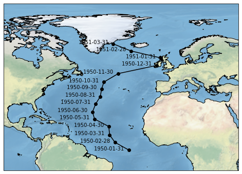
To select points along a transect defined in more then just lat-lon (trajectory). it is often convinient to use select_points method. Arrays defining a trajectory can directly be passed as arguments to select_points to make a trajectory like selection. However select method may also be used by using

advanced indexing of Xarray. Apart from this simplification, select_points also returns additional diagnostics related to point selection such as distance along the trajectory, that can be useful for plotting. In future we intend to add more diagnostics around selection like error estimates from selection.

import pandas as pd
# Define selection values in time, depth, lat, lon
sel_times = pd.date_range('1950-01-01', freq='M', periods=5)
sel_levels = [0, -10, -5, -30, -15]
sel_lats = np.linspace(-90,90,5)
sel_lons = np.linspace(-180,180,5)

fesom_ds.pyfesom2.select_points(lon=sel_lons, lat=sel_lats, nz1=sel_levels, time=sel_times)

<xarray.Dataset>
Dimensions:   (nod2: 5, nz: 48)
Coordinates:
    time      (nod2) datetime64[ns] 1950-01-31T23:15:00 ... 1950-05-31T23:15:00
    lat       (nod2) float64 dask.array<chunksize=(1,), meta=np.ndarray>
    lon       (nod2) float64 dask.array<chunksize=(1,), meta=np.ndarray>
    nz1       (nod2) float64 -2.5 -7.5 -2.5 -25.0 -15.0
  * nz        (nz) float64 0.0 -5.0 -10.0 -20.0 ... -5.65e+03 -6e+03 -6.25e+03
    distance  (nod2) float64 0.0 5.017e+03 1.503e+04 2.504e+04 3.005e+04
Dimensions without coordinates: nod2
Data variables:
    temp      (nod2) float32 dask.array<chunksize=(5,), meta=np.ndarray>
    salt      (nod2) float32 dask.array<chunksize=(5,), meta=np.ndarray>
    a_ice     (nod2) float32 dask.array<chunksize=(5,), meta=np.ndarray>
    m_ice     (nod2) float32 dask.array<chunksize=(5,), meta=np.ndarray>
    ssh       (nod2) float32 dask.array<chunksize=(5,), meta=np.ndarray>
    sst       (nod2) float32 dask.array<chunksize=(5,), meta=np.ndarray>
Attributes:
    Dataset URL:  https://swiftbrowser.dkrz.de/public/dkrz_02942825-0cab-44f3...

Note in such trajectory selection, all the dimensions used as indexers need to be of same size. The return dataset has these selected indexers on a common dimentions nod2. See accessor_plotting.ipynb example for opinionated ploting such transect.

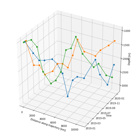
3. Advanced selections

Both select and select_points methods support Xarray’s advanced indexing, this can be leveraged to select multiple trajectories at once. To use Xarray’s advanced indexing, indexers have to be defined as dataarrays with a common dimentions.

Define three sample trajectories in lat, lon, time and depth.

import xarray as xr
lons_ref = np.array([-25., -33., -36., -37., -45])
lons = xr.DataArray([lons_ref, lons_ref-5., lons_ref+5.], dims=('ntraj', 'trajectory'))

lats_ref = [ 2.,  7., 11. , 16., 20.]
lats = xr.DataArray([lats_ref, lats_ref, lats_ref], dims=('ntraj', 'trajectory'))

levs = np.array([[-800., -700., -750., -900., -950.],
                 [-800., -500., -400., -600., -700.],
                 [-800., -900., -750., -600., -700.]])
levs = xr.DataArray(levs, dims=('ntraj', 'trajectory'))

times_ref = pd.date_range('1950-01-01', freq='M', periods=5)
times = xr.DataArray([times_ref, times_ref, times_ref], dims=('ntraj', 'trajectory'))

Select the trajectories at once. Dimension ntraj can be used to identify the trajectory.

fesom_ds.pyfesom2.select_points(lon=lons, lat=lats, time =times, nz1=levs)

<xarray.Dataset>
Dimensions:   (ntraj: 3, nz: 48, trajectory: 5)
Coordinates:
    time      (ntraj, trajectory) datetime64[ns] 1950-01-31T23:15:00 ... 1950...
    lat       (ntraj, trajectory) float64 dask.array<chunksize=(3, 5), meta=np.ndarray>
    lon       (ntraj, trajectory) float64 dask.array<chunksize=(3, 5), meta=np.ndarray>
    nz1       (ntraj, trajectory) float64 -850.0 -735.0 -735.0 ... -630.0 -735.0
  * nz        (nz) float64 0.0 -5.0 -10.0 -20.0 ... -5.65e+03 -6e+03 -6.25e+03
    distance  (ntraj, trajectory) float64 0.0 1.046e+06 ... 2.161e+06 3.117e+06
Dimensions without coordinates: ntraj, trajectory
Data variables:
    temp      (ntraj, trajectory) float32 dask.array<chunksize=(3, 5), meta=np.ndarray>
    salt      (ntraj, trajectory) float32 dask.array<chunksize=(3, 5), meta=np.ndarray>
    a_ice     (ntraj, trajectory) float32 dask.array<chunksize=(3, 5), meta=np.ndarray>
    m_ice     (ntraj, trajectory) float32 dask.array<chunksize=(3, 5), meta=np.ndarray>
    ssh       (ntraj, trajectory) float32 dask.array<chunksize=(3, 5), meta=np.ndarray>
    sst       (ntraj, trajectory) float32 dask.array<chunksize=(3, 5), meta=np.ndarray>
Attributes:
    Dataset URL:  https://swiftbrowser.dkrz.de/public/dkrz_02942825-0cab-44f3...

4. Selection on variables

In above examples selections were performed on entire dataset, which is convininent to make selections on entire dataset but the .pyfesom2 accessor can also be used on individual data variables (dataarrays) of datasets.

fesom_ds.pyfesom2.temp.select_points(lon=sel_lons, lat=sel_lats, nz1=sel_levels)

<xarray.DataArray 'temp' (time: 144, nod2: 5)>
dask.array<transpose, shape=(144, 5), dtype=float32, chunksize=(1, 5), chunktype=numpy.ndarray>
Coordinates:
  * time      (time) datetime64[ns] 1948-01-31T23:15:00 ... 1959-12-31T23:15:00
    lat       (nod2) float64 dask.array<chunksize=(1,), meta=np.ndarray>
    lon       (nod2) float64 dask.array<chunksize=(1,), meta=np.ndarray>
    nz1       (nod2) float64 -2.5 -7.5 -2.5 -25.0 -15.0
    distance  (nod2) float64 0.0 5.017e+03 1.503e+04 2.504e+04 3.005e+04
Dimensions without coordinates: nod2
Attributes:
    description:  temperature
    units:        C

Here select_points is used on variable temp to select a transect defined using sel_lons, sel_lats and sel_levs.

Region selection on a data variable returns an Xarray dataset. This is unlike selection on data variables in Xarray, which always returns a dataarray. Returning dataset for region selection was necessary to retain faces coordinate variable which otherwise would not be not possible to retain in a dataarray. The coordinate variable faces is necessary for spatial plots and to be able to save the region subset as a standalone dataset.