This page was generated from notebooks/plot_main.ipynb. Interactive online version: .

Visualizing FESOM2.0 simulations

%matplotlib inline
%load_ext autoreload
%autoreload 2

## import standard python packages

# import standard python packages
import sys
import numpy as np
import os
# import basemap
# from mpl_toolkits.basemap import Basemap
# import FESOM packages
sys.path.append("../")
from pyfesom2 import load_mesh, ind_for_depth, read_fesom_slice, ftriplot, fesom2clim, wplot_xy, read_fesom_sect
# from load_mesh_data import *
# from regriding import fesom2clim
# sys.path.append("/home/h/hbkdsido/utils/seawater-1.1/")
# import seawater as sw
# from fesom_plot_tools import *
from netCDF4 import Dataset
import cmocean.cm as cmo
import matplotlib
import matplotlib.pylab as plt
fontsize=20
matplotlib.rc('xtick', labelsize=fontsize)
matplotlib.rc('ytick', labelsize=fontsize)

Read the mesh

from mpl_toolkits.basemap import Basemap

# set the path to the mesh
#meshpath  ='/home/ollie/nkolduno/meshes/pi-grid/'
meshpath  ='/Users/koldunovn/PYHTON/DATA/CORE_MESH'
#meshpath  ='/work/ollie/ogurses/NATMAP/mesh_F2GLO08/'
alpha, beta, gamma=[50, 15, -90]
#alpha, beta, gamma=[0, 0, 0]
try:
    mesh
except NameError:
    print("mesh will be loaded")
    mesh=load_mesh(meshpath, abg=[alpha, beta, gamma], usepickle = False)
else:
    print("mesh with this name already exists and will not be loaded")

mesh with this name already exists and will not be loaded

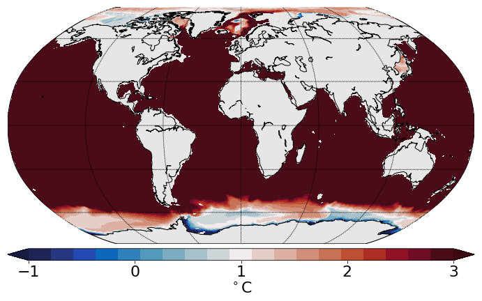
Example 1: plot the 2D slice of data at depth

# set the paths to the results, runid, etc.
result_path ='/Users/koldunovn/PYHTON/DATA/CORE_out/'
runid ='fesom'
str_id='temp'

# specify depth, records and year to read
depth, records, year=300, np.linspace(0,0,1).astype(int), 2000

# set the label for the colorbar & contour intervals for ftriplot
cbartext, cont = '$^\circ$C', [-1., 3., .1]

# get the closest model depth to the desired one
ilev=ind_for_depth(depth, mesh)

# read the model result from str_id.XXXX.nc
data=read_fesom_slice(str_id, records, year, mesh, result_path, runid, ilev=ilev)

# choose the colorbar and plot the data
cmap=cmo.balance
fig =plt.figure(figsize=(12,8))

# ftriplot is defined in fesom_plot_tools.py
data[data==0]=np.nan
[im, map, cbar]=ftriplot(mesh, data, np.linspace(cont[0], cont[1], 20), oce='global', cmap=cmap)
cbar.set_label(cbartext, fontsize=22)
cbar.set_ticks([round(i,7) for i in np.linspace(cont[0], cont[1], 5)])
cbar.ax.tick_params(labelsize=22)

ftriplot, number of dummy points: 67455

/Users/koldunovn/PYHTON/pyfesom2/pyfesom2/fesom_plot_tools.py:53: RuntimeWarning: invalid value encountered in less_equal
  data2[data2<=contours.min()]=contours.min()+eps
/Users/koldunovn/PYHTON/pyfesom2/pyfesom2/fesom_plot_tools.py:54: RuntimeWarning: invalid value encountered in greater_equal
  data2[data2>=contours.max()]=contours.max()-eps

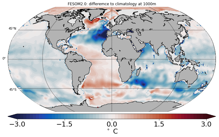
Example 2: Comparing to Climatology

# read the climatology
from pyfesom2 import climatology
phc=climatology('/Users/koldunovn/PYHTON/DATA/climatology/phc3.0_winter.nc')

# set the paths to the results, runid, etc.
result_path ='/Users/koldunovn/PYHTON/DATA/CORE_out/'
runid ='fesom'
str_id='temp'

# specify depth, records and year to read
depth, records, year=1000, np.linspace(0,0,1).astype(int), 2000

# set the label for the colorbar & contour intervals for ftriplot
cbartext, cont = '$^\circ$C', [-3., 3., .1]

# get the closest model depth to the desired one
ilev=ind_for_depth(depth, mesh)

# read the model result from str_id.XXXX.nc
data=read_fesom_slice(str_id, records, year, mesh, result_path, runid, ilev=ilev)

# interpolate the data onto the climatology grig
[iz, xx, yy, zz]=fesom2clim(data, depth, mesh, phc, radius_of_influence=10000000)

# plot the difference to climatology
cbartext=('$^\circ$ C' if (str_id=='temp') else 'psu')

# compute the difference to climatology (only T & S are supported)
dd=zz[:,:]-(phc.T[iz,:,:] if (str_id=='temp') else phc.S[iz,:,:])

# choose the colorbar and plot the data
cmap=cmo.balance

# wplot_xy is defined in fesom_plot_tools.py
fig = plt.figure(figsize=(12,8))
[im, map, cbar]=wplot_xy(xx,yy,dd,np.arange(cont[0], cont[1]+cont[2], cont[2]), cmap=cmap, do_cbar=True)
cbar.set_label(cbartext, fontsize=22)
cbar.set_ticks([round(i,4) for i in np.linspace(cont[0], cont[1], 5)])
cbar.ax.tick_params(labelsize=22)
plt.title('FESOM2.0: differemce to climatology at ' + np.str(depth)+'m')

/Users/koldunovn/PYHTON/pyfesom2/pyfesom2/climatology.py:60: RuntimeWarning: invalid value encountered in greater
  self.T = np.copy(ncfile.variables['temp'][:,:,:])
/Users/koldunovn/PYHTON/pyfesom2/pyfesom2/climatology.py:69: RuntimeWarning: invalid value encountered in greater
  self.S=np.copy(ncfile.variables['salt'][:,:,:])
/Users/koldunovn/PYHTON/pyfesom2/pyfesom2/climatology.py:77: RuntimeWarning: Mean of empty slice
  self.Tyz=nanmean(self.T, 2)
/Users/koldunovn/PYHTON/pyfesom2/pyfesom2/climatology.py:78: RuntimeWarning: Mean of empty slice
  self.Syz=nanmean(self.S, 2)

the model depth is:  1000 ; the closest depth in climatology is:  1000.0

/Users/koldunovn/PYHTON/pyfesom2/pyfesom2/fesom_plot_tools.py:118: RuntimeWarning: invalid value encountered in less_equal
  zz[zz<=contours.min()]=contours.min()+eps
/Users/koldunovn/PYHTON/pyfesom2/pyfesom2/fesom_plot_tools.py:119: RuntimeWarning: invalid value encountered in greater_equal
  zz[zz>=contours.max()]=contours.max()-eps

<matplotlib.text.Text at 0x11241a978>

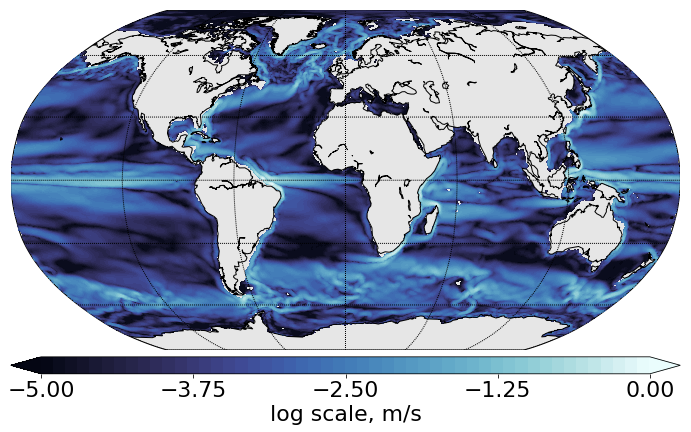
Example 3: Plot the norm of velocity (given on elements)

from numba import jit
@jit("float64[:](float64[:],int64, float64[:], int64[:,:], int64, float64[:])", nopython=True)
def tonodes(component, n2d, voltri, elem, e2d, lump2):
    ''' Function to interpolate from elements to nodes.
    Made fast with numba.
    '''
    onnodes=np.zeros(shape=n2d)

    var_elem=component*voltri
    for i in range(e2d):
        onnodes[elem[i,:]]=onnodes[elem[i,:]]+np.array([var_elem[i], var_elem[i], var_elem[i]])
    onnodes=onnodes/lump2/3.
    return onnodes

# set the paths to the results, runid, etc.
result_path ='/Users/koldunovn/PYHTON/DATA/CORE_out/'
runid ='fesom'

# specify depth, records and year to read
depth, records, year=100, np.linspace(0,0,1).astype(int), 2000

# set the label for the colorbar & contour intervals for ftriplot
cbartext, cont = 'log scale, m/s', [-5.,0., 0.1]

# get the closest model depth to the desired one
ilev=ind_for_depth(depth, mesh)

# read the ocean velocities
u=read_fesom_slice('u', records, year, mesh, result_path, runid, ilev=ilev)
v=read_fesom_slice('v', records, year, mesh, result_path, runid, ilev=ilev)
# one could use Dataset instead:
# f=Dataset('../results/run_8km_noGMHO/fesom.1960.oce.restart.nc')
# u=f.variables['u'][0,:,11]
# v=f.variables['v'][0,:,11]

# velocities on elements will be interpolated onto nodes
# allocate the nodal fields
unodes=np.zeros(shape=mesh.n2d)
vnodes=np.zeros(shape=mesh.n2d)

#  old and slow way to interpolate original velocities onto nods (unodes, vnodes)
# var_elem=u*mesh.voltri
# for i in range(mesh.e2d):
#     unodes[mesh.elem[i,:]]=unodes[mesh.elem[i,:]]+[var_elem[i], var_elem[i], var_elem[i]]
# unodes=unodes/mesh.lump2/3.

# var_elem=v*mesh.voltri
# for i in range(mesh.e2d):
#     vnodes[mesh.elem[i,:]]=vnodes[mesh.elem[i,:]]+[var_elem[i], var_elem[i], var_elem[i]]
# vnodes=vnodes/mesh.lump2/3.

#  new and fast way to interpolate original velocities onto nods (unodes, vnodes). Require numba.
unodes = tonodes(u, mesh.n2d, mesh.voltri, mesh.elem, mesh.e2d, mesh.lump2)
vnodes = tonodes(v, mesh.n2d, mesh.voltri, mesh.elem, mesh.e2d, mesh.lump2)

# compute the absolute velocity
data=np.hypot(unodes, vnodes)

# plot the result
cmap=cmo.ice
fig = plt.figure(figsize=(12,8))
# ftriplot is defined in fesom_plot_tools.py
data[data==0]=np.nan
[im, map, cbar]=ftriplot(mesh, np.log(data), np.arange(cont[0], cont[1]+cont[2], cont[2]), oce='global', cmap=cmap)
cbar.set_label(cbartext, fontsize=22)
cbar.set_ticks([round(i,4) for i in np.linspace(cont[0], cont[1], 5)])
cbar.ax.tick_params(labelsize=22)

ftriplot, number of dummy points: 48065

/Users/koldunovn/PYHTON/pyfesom2/pyfesom2/fesom_plot_tools.py:53: RuntimeWarning: invalid value encountered in less_equal
  data2[data2<=contours.min()]=contours.min()+eps
/Users/koldunovn/PYHTON/pyfesom2/pyfesom2/fesom_plot_tools.py:54: RuntimeWarning: invalid value encountered in greater_equal
  data2[data2>=contours.max()]=contours.max()-eps

Example 4: Plot a section

# set the paths to the results, runid, etc.
result_path ='/Users/koldunovn/PYHTON/DATA/CORE_out/'
runid ='fesom'
str_id='temp'

# specify records and year to read
records, year=np.linspace(0,0,1).astype(int), 2000

# set the label for the colorbar & contour intervals for ftriplot
cbartext, cont = '$^\circ$C', [1., 30., .1]

# define the section with points p1(x1,y1), p2(x2,y2)
p1=np.array([-30.,   -80.])
p2=np.array([-30.,    90.])

# set the number of descrete points in horizontal and vertical (nxy and nz, respectively) to represent the section
nxy=100
nz =46

# read thesection from the data
[sx, sy, sz]=read_fesom_sect(str_id, records, year, mesh, result_path, runid, p1, p2, nxy, nz, \
    how='mean', line_distance=5., radius_of_influence=300000)

# replace dummies with NaNs
sz[sz>1.e100]=np.nan

# plot the result
cmap=cmo.balance
fig = plt.figure(figsize=(12,8))
plt.contourf(sy, mesh.zlev[0:nz], sz, cmap=cmap, levels=np.linspace(cont[0], cont[1], 50), extend='both')
plt.xlabel('distance, [degree]', fontsize=fontsize)
plt.ylabel('depth, [m]', fontsize=fontsize)
cbar=plt.colorbar(orientation="horizontal", pad=.2)
cbar.set_ticks([round(i,4) for i in np.linspace(cont[0], cont[1], 5)])
cbar.set_label(cbartext, fontsize=fontsize)
cbar.set_label(cbartext, fontsize=fontsize)

/Users/koldunovn/miniconda3/lib/python3.6/site-packages/pyresample/kd_tree.py:397: UserWarning: Possible more than 10 neighbours within 300000 m for some data points
  (neighbours, radius_of_influence))
/Users/koldunovn/miniconda3/lib/python3.6/site-packages/ipykernel_launcher.py:24: RuntimeWarning: invalid value encountered in greater

Example 5: Computing MOC from vertical velocity

# set the paths to the results, runid, etc.
result_path ='/Users/koldunovn/PYHTON/DATA/CORE_out/'
runid ='fesom'

# set the label for the colorbar & contour intervals for ftriplot
cbartext, cont = 'Sv', [-30., 30., .5]

# define a descrete set of latitudes
nlats=91
lats=np.linspace(-90, 90, nlats)
dlat=lats[1]-lats[0]
# allocate moc array
moc=np.zeros([mesh.nlev, nlats])

# read the required metadata (mesh diagnostic file is always created at the cold start)
# grid information is needed for computing the MOC
ncfile  = Dataset(os.path.join(result_path, runid+'.mesh.diag.nc'))
el_area =ncfile.variables['elem_area'][:]
nlevels =ncfile.variables['nlevels'][:]-1
el_nodes=ncfile.variables['elem'][:,:]-1
nodes_x =ncfile.variables['nodes'][0,:]*180./np.pi
nodes_y =ncfile.variables['nodes'][1,:]*180./np.pi

# compute lon/lat coordinate of an element required lated for binning
elem_x  =nodes_x[el_nodes].sum(axis=0)/3.
elem_y  =nodes_y[el_nodes].sum(axis=0)/3.

# specify records and year to read
records, year=np.linspace(0,0,1).astype(int), 2000

# compute MOC
# precompute positions of elements for binning
pos = ((elem_y-lats[0])/dlat).astype('int')

# compute contributions from vertical velocities on elements and put them into bins
for i in range(mesh.nlev):
# read the model result from fesom.XXXX.oce.nc
    w=read_fesom_slice('w', records, year, mesh, result_path, runid, ilev=i)
#     print(i)
    # mean over elements
    elem_mean = np.sum(w[el_nodes[:,:]], axis=0)/3.*1.e-6
    # weigh by element area
    elem_mean_weigh = el_area*elem_mean
    # select nodes to consider in calculation based on number of levels
    toproc = np.where(i <=  nlevels-1)[0]
    # for every bin select elements that belong to the bin and sum them.
    for k in range(pos.min(), pos.max()+1):
#         if (i <= nlevels[e]-1):
            moc[i, k]=elem_mean_weigh[toproc][pos[toproc]==k].sum()

# the result from the previous step needs to be cumulatively summed
moc = np.ma.cumsum(np.ma.masked_invalid(moc), axis=1)

# plot the result
cmap=cmo.balance
fig = plt.figure(figsize=(10,6))
plt.contourf(lats, mesh.zlev, moc, cmap=cmap, levels=np.linspace(cont[0], cont[1], 50), extend='both')
plt.xlabel('latitude, [degree]', fontsize=fontsize)
plt.ylabel('depth, [m]', fontsize=fontsize)
cbar=plt.colorbar(orientation="horizontal", pad=.2)
cbar.set_ticks([round(i,4) for i in np.linspace(cont[0], cont[1], 5)])
cbar.set_label(cbartext, fontsize=fontsize)
cbar.set_label(cbartext, fontsize=fontsize)

---------------------------------------------------------------------------
FileNotFoundError                         Traceback (most recent call last)
<ipython-input-31-896ec64de4bb> in <module>()
     36 for i in range(mesh.nlev):
     37 # read the model result from fesom.XXXX.oce.nc
---> 38     w=read_fesom_slice('w', records, year, mesh, result_path, runid, ilev=i)
     39 #     print(i)
     40     # mean over elements

~/PYHTON/pyfesom2/pyfesom2/load_mesh_data.py in read_fesom_slice(str_id, records, year, mesh, result_path, runid, ilev, how, verbose, ncfile)
    279     if (verbose):
    280         print(['reading ', ncfile])
--> 281     f = Dataset(ncfile, 'r')
    282     # dimensions of the netcdf variable
    283     ncdims=f.variables[str_id].shape

netCDF4/_netCDF4.pyx in netCDF4._netCDF4.Dataset.__init__()

netCDF4/_netCDF4.pyx in netCDF4._netCDF4._ensure_nc_success()

FileNotFoundError: [Errno 2] No such file or directory: b'/Users/koldunovn/PYHTON/DATA/CORE_out//w.fesom.2000.nc'

Auxuary things, manipulations with the topography

closing the Gibraltar Strait by setting the depth there to 20m

!mesh needs to be repartitioned afterwards!

# find nodes around Gibraltar
ind=(mesh.x2 > -6.5) & (mesh.x2 < -3.5) & (mesh.y2 > 34.5) & (mesh.y2 < 37.5)
ind=[i for (i, val) in enumerate(ind) if (val)]

# read mesh topography from file (in case we do not trust already loaded mesh information data)
topofile='/work/ollie/dsidoren/input/fesom2.0/meshes/mesh_CORE2_final/aux3d.out'
with open(topofile) as f:
     nlev=int(next(f))
     zlev=np.array([next(f).rstrip() for x in range(nlev)]).astype(float)
     topo=np.array([next(f).rstrip() for x in range(mesh.n2d)]).astype(float)

# set depth around Gibraltar to 20m and save it into different mesh file
topo[ind]=topo[ind]=-20.

# create the new aux3d.out
topofile_new='/work/ollie/dsidoren/input/fesom2.0/meshes/mesh_CORE2_final/aux3d.out.new'
f = open(topofile_new, 'w')
f.write(str(nlev)+'\n')
for depth in zlev:
    f.write(str(depth)+'\n')
for depth in topo:
    f.write(str(depth)+'\n')
f.close()

increasing the amount of vertical levels to that from NEMO (74 levels)

read the prepared on the mesh etopo5 topography

skip the second and third level in order do improve CFL

!mesh needs to be repartitioned afterwards!

meshpath  ='/work/ollie/dsidoren/input/fesom2.0/meshes/mesh_CORE2_final/'
nf=Dataset(meshpath+'etopo.nc') # ETOPO5 topography already prepared
topo=nf.variables['topo'][:]
topo[topo >=     0]=-10.
topo[topo < -6500]=-6500.
# read the NEMO 74 vertical levels
nf=Dataset('/work/ollie/dsidoren/input/fesom2.0/NEMO_levels74.nc')
levels=-nf.variables['gdepw_0'][0,:]
# skip the very upper except for the first leveld in order to improve CFL
# add more depths
levels=np.concatenate((levels[[0, 4]], levels[5:], np.array([levels[-1]+levels[-1]-levels[-2], -6250])))
N=len(levels)

# create the new aux3d.out
topofile_new='/work/ollie/dsidoren/input/fesom2.0/meshes/mesh_CORE2_final/aux3d.out.etopo5N74'
f = open(topofile_new, 'w')
f.write(str(N)+'\n')
for depth in levels:
    f.write(str(depth)+'\n')
for depth in topo:
    f.write(str(depth)+'\n')
f.close()