Pyfesom2 Overview
Pyfesom2 is python model for working with FESOM2 data. The FESOM2 is different from other ocean models by supporting unstructured triangular meshes of variable resolution.
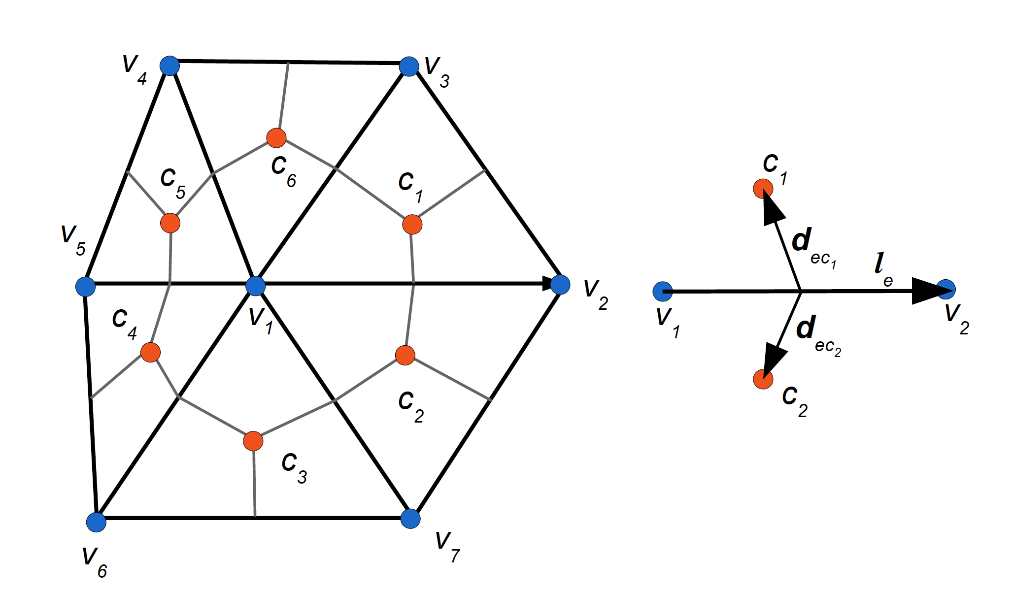
The mesh is defined as a collection of points (vertices, or nodes) shown as blue dots, and connections between this points. More details about the geometry: https://fesom2.readthedocs.io/en/latest/geometry.html and mesh itself: https://fesom2.readthedocs.io/en/latest/meshes/meshes.html
Download and installation
pyfesom2
GitHub: https://github.com/FESOM/pyfesom2
Installation instructions: https://github.com/FESOM/pyfesom2/blob/master/README.md
Data and mesh
If you would like to try to repeat examples from this introduction, you can download FESOM2 data and mesh. The data are quite heavy, about 15 Gb.
Link: https://swiftbrowser.dkrz.de/public/dkrz_c719fbc3-98ea-446c-8e01-356dac22ed90/PYFESOM2/
You have to download both archives (LCORE.tar and LCORE_MESH.tar) and extract them.
Alternative would be to use very light weight mesh that comes with pyfesom2 in the tests/data/pi-grid/ and example data on this mesh in tests/data/pi-results.
Command line utilities
Most of the visualisation tools, like ncview, work with gridded regular data. We can interpolate FESOM2 data to regular grid to make use of all this tools. Many analysis can be also done with gridded data. If pyfesom is installed with pip install -e ., you will have two comand line tools available:
pfinterp
pfplot
pfinterp
The most useful for most people would be the pfinterp. As a minimum you should provide path to the mesh, path to the model ouptut and a variable name:
pfinterp /path/to/mesh/ /path/to/datafolder/ temp
by default pfinterp will search for the year 1948 and interpolate first time step from the depth 0 to a 1\(^\circ\) lon/lat regular grid.
pfinterp /Users/koldunovn/PYHTON/DATA/LCORE_MESH /Users/koldunovn/PYHTON/DATA/LCORE temp
Examples:
pfinterp /Users/koldunovn/PYHTON/DATA/LCORE_MESH /Users/koldunovn/PYHTON/DATA/LCORE temp -b -90 0 20 60 -r 360 160
pfinterp /Users/koldunovn/PYHTON/DATA/LCORE_MESH /Users/koldunovn/PYHTON/DATA/LCORE temp -y 1950:1952 -d 0,100,500 -r 1440 720 -i 40000 --interp idist -k 5 -o ./output.nc

# intepolates also vector values
pfinterp /Users/koldunovn/PYHTON/DATA/LCORE_MESH /Users/koldunovn/PYHTON/DATA/LCORE u -y 1950 -d 100 -o ./u.nc

# fast
pfinterp /Users/koldunovn/PYHTON/DATA/LCORE_MESH /Users/koldunovn/PYHTON/DATA/LCORE a_ice -y 1950:1952 -d 0 -r 1440 720 -i 120000  -o ./a_ice.nc
Documentation: https://pyfesom2.readthedocs.io/en/latest/pfinterp.html
pfplot
Plots scalar from FESOM mesh interpolated on regular grid. Sometimes can be usefull if you need to explore the data a bit more interactivelly.
Examples:
pfplot /Users/koldunovn/PYHTON/DATA/LCORE_MESH /Users/koldunovn/PYHTON/DATA/LCORE temp -y 1950:1952 -d 0 -r 1440 720 -i 120000 --interp nn
Documentation: https://pyfesom2.readthedocs.io/en/latest/pfplot.html
pyfesom2 basic functionality
[1]:
import pyfesom2 as pf
Loading the mesh
[2]:
mesh = pf.load_mesh('/Users/koldunovn/PYHTON/DATA/LCORE_MESH/',
                    abg=[50, 15, -90])
/Users/koldunovn/PYHTON/DATA/LCORE_MESH/pickle_mesh_py3_fesom2
The usepickle == True)
The pickle file for FESOM2 exists.
The mesh will be loaded from /Users/koldunovn/PYHTON/DATA/LCORE_MESH/pickle_mesh_py3_fesom2
[3]:
mesh
[3]:
FESOM mesh:
path                  = /Users/koldunovn/PYHTON/DATA/LCORE_MESH
alpha, beta, gamma    = 50, 15, -90
number of 2d nodes    = 126858
number of 2d elements = 244659
Three main things you need in the mesh object are:
[4]:
mesh.x2
[4]:
array([ 110.8836505 , -102.42504166,  -43.16270946, ...,  -25.06347164,
        -78.51742993,  -78.28109577])
[5]:
mesh.y2
[5]:
array([-66.14835661, -74.21462105, -77.60296032, ..., -74.57136759,
        24.57448735,  25.02531306])
[6]:
mesh.elem
[6]:
array([[  1763,  96635, 125225],
       [  1477, 112277,    703],
       [ 78543,  78544,   5048],
       ...,
       [ 94520, 126857,  94519],
       [ 94520, 126857,  94514],
       [126856,  19370,  94513]])
[7]:
mesh.x2[mesh.elem]
[7]:
array([[-153.23818726, -154.08441288, -153.99029711],
       [ -46.04259358,  -45.38235787,  -46.54028583],
       [-146.76658932, -147.63820606, -147.24055395],
       ...,
       [ -78.13578565,  -78.28109577,  -78.66768799],
       [ -78.13578565,  -78.28109577,  -77.81496951],
       [ -78.51742993,  -78.8651748 ,  -78.55601404]])
Loading the data
[8]:
data = pf.get_data("/Users/koldunovn/PYHTON/DATA/LCORE/", "temp", 1950, mesh)
Depth is None, 3d field will be returned
[9]:
mesh
[9]:
FESOM mesh:
path                  = /Users/koldunovn/PYHTON/DATA/LCORE_MESH
alpha, beta, gamma    = 50, 15, -90
number of 2d nodes    = 126858
number of 2d elements = 244659
[10]:
data.shape
[10]:
(126858, 47)
[11]:
data = pf.get_data("/Users/koldunovn/PYHTON/DATA/LCORE/", "temp", range(1950,1952), mesh)
Depth is None, 3d field will be returned
[12]:
data.shape
[12]:
(126858, 47)
[13]:
data = pf.get_data("/Users/koldunovn/PYHTON/DATA/LCORE/", "temp", [1950, 1951, 1952], mesh, how=None)
Depth is None, 3d field will be returned
[14]:
data.shape
[14]:
(3, 126858, 47)
[15]:
data = pf.get_data("/Users/koldunovn/PYHTON/DATA/LCORE/", "temp", range(1950,1952), mesh, how=None, compute=False)
Depth is None, 3d field will be returned
[16]:
data
[16]:
- time: 2
- nod2: 126858
- nz1: 47
- dask.array<chunksize=(1, 126858, 47), meta=np.ndarray>
Array Chunk Bytes 47.70 MB 23.85 MB Shape (2, 126858, 47) (1, 126858, 47) Count 6 Tasks 2 Chunks Type float32 numpy.ndarray - time(time)datetime64[ns]1950-12-31T23:15:00 1951-12-31T23:15:00
- long_name :
- time
array(['1950-12-31T23:15:00.000000000', '1951-12-31T23:15:00.000000000'],
      dtype='datetime64[ns]')
- description :
- temperature
- units :
- C
[17]:
data = pf.get_data("/Users/koldunovn/PYHTON/DATA/LCORE/",
                   "temp",
                   range(1950,1952),
                   mesh,
                   how='ori',
                   compute=False,
                  chunks={'nod2':10000, 'nz1':5})
Depth is None, 3d field will be returned
[18]:
data
[18]:
- time: 2
- nod2: 126858
- nz1: 47
- dask.array<chunksize=(1, 10000, 5), meta=np.ndarray>
Array Chunk Bytes 47.70 MB 200.00 kB Shape (2, 126858, 47) (1, 10000, 5) Count 522 Tasks 260 Chunks Type float32 numpy.ndarray - time(time)datetime64[ns]1950-12-31T23:15:00 1951-12-31T23:15:00
- long_name :
- time
array(['1950-12-31T23:15:00.000000000', '1951-12-31T23:15:00.000000000'],
      dtype='datetime64[ns]')
- description :
- temperature
- units :
- C
[19]:
data_mean = data.mean(dim='time').compute()
Plotting
[20]:
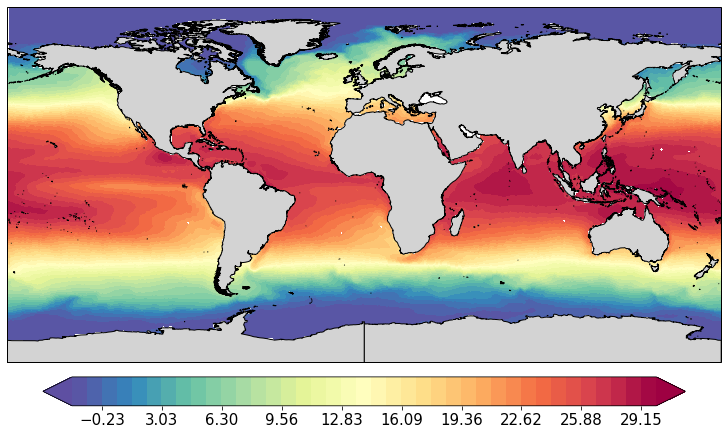
pf.plot(mesh, data_mean[:,0].values)
[20]:
[<cartopy.mpl.geoaxes.GeoAxesSubplot at 0x122891b38>]
[21]:
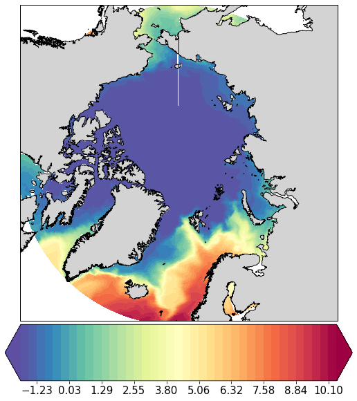
pf.plot(mesh, data_mean[:,0].values, mapproj='np', box=[-180, 180, 60, 90])
[21]:
[<cartopy.mpl.geoaxes.GeoAxesSubplot at 0x121c34a58>]
/Users/koldunovn/miniconda3/envs/pyfesom2/lib/python3.6/site-packages/IPython/core/pylabtools.py:128: UserWarning: constrained_layout not applied.  At least one axes collapsed to zero width or height.
  fig.canvas.print_figure(bytes_io, **kw)
[22]:
data2_mean = pf.get_data("/Users/koldunovn/PYHTON/DATA/LCORE/",
                   "temp",
                   range(1952,1954),
                   mesh,
                   how='mean',
                   compute=True)
Depth is None, 3d field will be returned
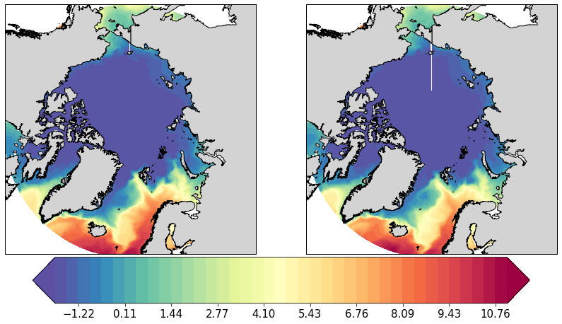
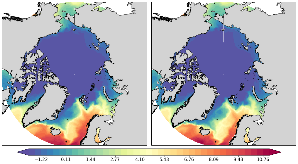
[24]:
pf.plot(mesh,
        [data_mean[:,0].values, data2_mean[:,0]] ,
        mapproj='np',
        box=[-180, 180, 60, 90],
       rowscol=[1,2],
       figsize=(14,8))
[24]:
array([<cartopy.mpl.geoaxes.GeoAxesSubplot object at 0x1227e65c0>,
       <cartopy.mpl.geoaxes.GeoAxesSubplot object at 0x1227fd5f8>],
      dtype=object)
[25]:
import matplotlib.pylab as plt
[26]:
pf.plot(mesh,
        [data_mean[:,0].values, data2_mean[:,0]] ,
        mapproj='np',
        box=[-180, 180, 60, 90],
       rowscol=[1,2],
       figsize=(14,8))
plt.savefig('test.png')
/Users/koldunovn/miniconda3/envs/pyfesom2/lib/python3.6/site-packages/ipykernel_launcher.py:7: UserWarning: constrained_layout not applied.  At least one axes collapsed to zero width or height.
  import sys
[27]:
import matplotlib.cm as cm
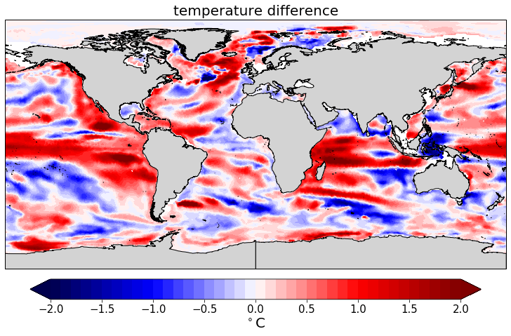
[28]:
pf.plot(mesh,
        data2_mean[:,11] - data_mean[:,11].values,
        cmap=cm.seismic,
        levels=(-2,2,41),
        units=r'$^\circ$C',
        titles='temperature difference',
       )
[28]:
[<cartopy.mpl.geoaxes.GeoAxesSubplot at 0x122acfc18>]
Plotting Transects
[29]:
temp = pf.get_data('/Users/koldunovn/PYHTON/DATA/LCORE/', 'temp', [1950], mesh)
Depth is None, 3d field will be returned
[30]:
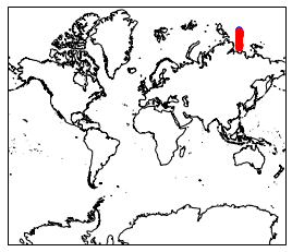
lon_start = 120
lat_start = 75
lon_end = 120
lat_end = 80
npoints   = 50
lonlat = pf.transect_get_lonlat(lon_start, lat_start, lon_end, lat_end, npoints)
[31]:
pf.plot_transect_map(lonlat, mesh, view='w')
[31]:
<cartopy.mpl.geoaxes.GeoAxesSubplot at 0x128bd6e48>
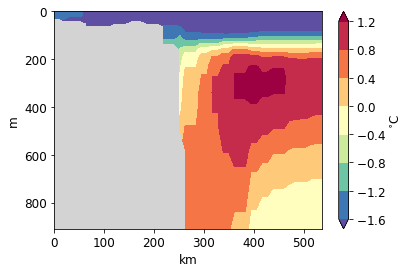
[32]:
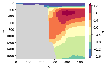
pf.plot_transect(
    temp,
    mesh,
    lonlat,
)
[32]:
<matplotlib.contour.QuadContourSet at 0x122a9a4a8>
[33]:
pf.plot_transect(
    temp,
    mesh,
    lonlat,
    maxdepth=2000,
)
[33]:
<matplotlib.contour.QuadContourSet at 0x1229fab38>
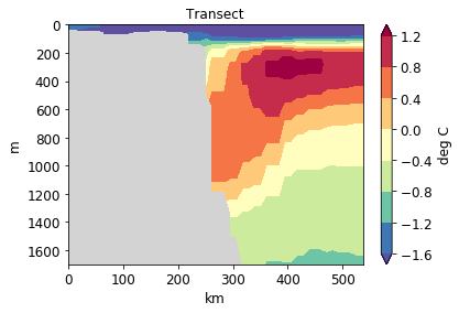
[34]:
pf.plot_transect(
    temp,
    mesh,
    lonlat,
    maxdepth=2000,
    label="deg C",
    title="Transect",
)
[34]:
<matplotlib.contour.QuadContourSet at 0x1229d9550>
[35]:
import numpy as np
[36]:
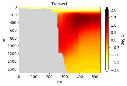
pf.plot_transect(
    temp,
    mesh,
    lonlat,
    maxdepth=2000,
    label="deg C",
    title="Transect",
    levels=np.linspace(-2,2, 41),
    cmap=cm.hot_r,
)
[36]:
<matplotlib.contour.QuadContourSet at 0x122a3ddd8>
[37]:
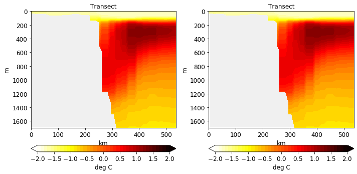
pf.plot_transect(
    [temp, temp],
    mesh,
    lonlat,
    maxdepth=2000,
    label="deg C",
    title="Transect",
    levels=np.linspace(-2,2, 41),
    cmap=cm.hot_r,
    ncols=2,
    figsize=(10,5),
    facecolor='#f0f0f0'
)
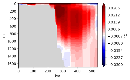
U/V transect
[38]:
u = pf.get_data('/Users/koldunovn/PYHTON/DATA/LCORE/', 'u', [1955], mesh)
v = pf.get_data('/Users/koldunovn/PYHTON/DATA/LCORE/', 'v', [1955], mesh)
Depth is None, 3d field will be returned
Depth is None, 3d field will be returned
[39]:
u.shape
[39]:
(244659, 47)
[40]:
u_nodes = pf.tonodes3d(u, mesh)
v_nodes = pf.tonodes3d(v, mesh)
[41]:
lon_start = 120
lat_start = 75
lon_end = 120
lat_end = 80
lonlat = pf.transect_get_lonlat(lon_start, lat_start, lon_end, lat_end, npoints)
[42]:
rot_u, rot_v, dist, nodes = pf.transect_uv(u_nodes, v_nodes, mesh, lon_start, lat_start, lon_end, lat_end, myangle=0,
                                           max_distance=30000, npoints=npoints)
[43]:
pf.plot_transect(v_nodes,
                 mesh,
                 lonlat,
                 maxdepth=2000,
                 transect_data=rot_u.T,
                 dist=dist,
                 nodes=nodes,
                 levels= np.round(np.linspace(-0.03, 0.03, 42),4),
                 cmap=cm.seismic)
[43]:
<matplotlib.contour.QuadContourSet at 0x1298e7e48>
Diagnostics
Collection of diagnostics to easily repeat OMIP2 exersizes.
[44]:
import pyfesom2 as pf
[45]:
mesh = pf.load_mesh('/Users/koldunovn/PYHTON/DATA/LCORE_MESH/', abg=[50, 15, -90])
/Users/koldunovn/PYHTON/DATA/LCORE_MESH/pickle_mesh_py3_fesom2
The usepickle == True)
The pickle file for FESOM2 exists.
The mesh will be loaded from /Users/koldunovn/PYHTON/DATA/LCORE_MESH/pickle_mesh_py3_fesom2
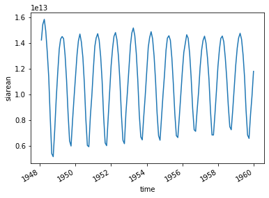
Sea ice integrals
[46]:
a_ice = pf.get_data('../../DATA/LCORE/', 'a_ice', range(1948,1960), mesh, how=None, compute=False)
Depth is None, 3d field will be returned
[47]:
a_ice
[47]:
- time: 144
- nod2: 126858
- dask.array<chunksize=(12, 126858), meta=np.ndarray>
Array Chunk Bytes 73.07 MB 6.09 MB Shape (144, 126858) (12, 126858) Count 36 Tasks 12 Chunks Type float32 numpy.ndarray - time(time)datetime64[ns]1948-01-31T23:15:00 ... 1959-12-31T23:15:00
- long_name :
- time
array(['1948-01-31T23:15:00.000000000', '1948-02-28T23:15:00.000000000',
       '1948-03-30T23:15:00.000000000', '1948-04-29T23:15:00.000000000',
       '1948-05-30T23:15:00.000000000', '1948-06-29T23:15:00.000000000',
       '1948-07-30T23:15:00.000000000', '1948-08-30T23:15:00.000000000',
       '1948-09-29T23:15:00.000000000', '1948-10-30T23:15:00.000000000',
       '1948-11-29T23:15:00.000000000', '1948-12-30T23:15:00.000000000',
       '1949-01-31T23:15:00.000000000', '1949-02-28T23:15:00.000000000',
       '1949-03-31T23:15:00.000000000', '1949-04-30T23:15:00.000000000',
       '1949-05-31T23:15:00.000000000', '1949-06-30T23:15:00.000000000',
       '1949-07-31T23:15:00.000000000', '1949-08-31T23:15:00.000000000',
       '1949-09-30T23:15:00.000000000', '1949-10-31T23:15:00.000000000',
       '1949-11-30T23:15:00.000000000', '1949-12-31T23:15:00.000000000',
       '1950-01-31T23:15:00.000000000', '1950-02-28T23:15:00.000000000',
       '1950-03-31T23:15:00.000000000', '1950-04-30T23:15:00.000000000',
       '1950-05-31T23:15:00.000000000', '1950-06-30T23:15:00.000000000',
       '1950-07-31T23:15:00.000000000', '1950-08-31T23:15:00.000000000',
       '1950-09-30T23:15:00.000000000', '1950-10-31T23:15:00.000000000',
       '1950-11-30T23:15:00.000000000', '1950-12-31T23:15:00.000000000',
       '1951-01-31T23:15:00.000000000', '1951-02-28T23:15:00.000000000',
       '1951-03-31T23:15:00.000000000', '1951-04-30T23:15:00.000000000',
       '1951-05-31T23:15:00.000000000', '1951-06-30T23:15:00.000000000',
       '1951-07-31T23:15:00.000000000', '1951-08-31T23:15:00.000000000',
       '1951-09-30T23:15:00.000000000', '1951-10-31T23:15:00.000000000',
       '1951-11-30T23:15:00.000000000', '1951-12-31T23:15:00.000000000',
       '1952-01-31T23:15:00.000000000', '1952-02-28T23:15:00.000000000',
       '1952-03-30T23:15:00.000000000', '1952-04-29T23:15:00.000000000',
       '1952-05-30T23:15:00.000000000', '1952-06-29T23:15:00.000000000',
       '1952-07-30T23:15:00.000000000', '1952-08-30T23:15:00.000000000',
       '1952-09-29T23:15:00.000000000', '1952-10-30T23:15:00.000000000',
       '1952-11-29T23:15:00.000000000', '1952-12-30T23:15:00.000000000',
       '1953-01-31T23:15:00.000000000', '1953-02-28T23:15:00.000000000',
       '1953-03-31T23:15:00.000000000', '1953-04-30T23:15:00.000000000',
       '1953-05-31T23:15:00.000000000', '1953-06-30T23:15:00.000000000',
       '1953-07-31T23:15:00.000000000', '1953-08-31T23:15:00.000000000',
       '1953-09-30T23:15:00.000000000', '1953-10-31T23:15:00.000000000',
       '1953-11-30T23:15:00.000000000', '1953-12-31T23:15:00.000000000',
       '1954-01-31T23:15:00.000000000', '1954-02-28T23:15:00.000000000',
       '1954-03-31T23:15:00.000000000', '1954-04-30T23:15:00.000000000',
       '1954-05-31T23:15:00.000000000', '1954-06-30T23:15:00.000000000',
       '1954-07-31T23:15:00.000000000', '1954-08-31T23:15:00.000000000',
       '1954-09-30T23:15:00.000000000', '1954-10-31T23:15:00.000000000',
       '1954-11-30T23:15:00.000000000', '1954-12-31T23:15:00.000000000',
       '1955-01-31T23:15:00.000000000', '1955-02-28T23:15:00.000000000',
       '1955-03-31T23:15:00.000000000', '1955-04-30T23:15:00.000000000',
       '1955-05-31T23:15:00.000000000', '1955-06-30T23:15:00.000000000',
       '1955-07-31T23:15:00.000000000', '1955-08-31T23:15:00.000000000',
       '1955-09-30T23:15:00.000000000', '1955-10-31T23:15:00.000000000',
       '1955-11-30T23:15:00.000000000', '1955-12-31T23:15:00.000000000',
       '1956-01-31T23:15:00.000000000', '1956-02-28T23:15:00.000000000',
       '1956-03-30T23:15:00.000000000', '1956-04-29T23:15:00.000000000',
       '1956-05-30T23:15:00.000000000', '1956-06-29T23:15:00.000000000',
       '1956-07-30T23:15:00.000000000', '1956-08-30T23:15:00.000000000',
       '1956-09-29T23:15:00.000000000', '1956-10-30T23:15:00.000000000',
       '1956-11-29T23:15:00.000000000', '1956-12-30T23:15:00.000000000',
       '1957-01-31T23:15:00.000000000', '1957-02-28T23:15:00.000000000',
       '1957-03-31T23:15:00.000000000', '1957-04-30T23:15:00.000000000',
       '1957-05-31T23:15:00.000000000', '1957-06-30T23:15:00.000000000',
       '1957-07-31T23:15:00.000000000', '1957-08-31T23:15:00.000000000',
       '1957-09-30T23:15:00.000000000', '1957-10-31T23:15:00.000000000',
       '1957-11-30T23:15:00.000000000', '1957-12-31T23:15:00.000000000',
       '1958-01-31T23:15:00.000000000', '1958-02-28T23:15:00.000000000',
       '1958-03-31T23:15:00.000000000', '1958-04-30T23:15:00.000000000',
       '1958-05-31T23:15:00.000000000', '1958-06-30T23:15:00.000000000',
       '1958-07-31T23:15:00.000000000', '1958-08-31T23:15:00.000000000',
       '1958-09-30T23:15:00.000000000', '1958-10-31T23:15:00.000000000',
       '1958-11-30T23:15:00.000000000', '1958-12-31T23:15:00.000000000',
       '1959-01-31T23:15:00.000000000', '1959-02-28T23:15:00.000000000',
       '1959-03-31T23:15:00.000000000', '1959-04-30T23:15:00.000000000',
       '1959-05-31T23:15:00.000000000', '1959-06-30T23:15:00.000000000',
       '1959-07-31T23:15:00.000000000', '1959-08-31T23:15:00.000000000',
       '1959-09-30T23:15:00.000000000', '1959-10-31T23:15:00.000000000',
       '1959-11-30T23:15:00.000000000', '1959-12-31T23:15:00.000000000'],
      dtype='datetime64[ns]')
- description :
- ice concentration
- units :
- %
[48]:
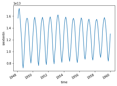
ice_area = pf.ice_area(a_ice, mesh,)
ice_ext = pf.ice_ext(a_ice, mesh)
[49]:
ice_area.plot()
[49]:
[<matplotlib.lines.Line2D at 0x12980d908>]
[50]:
ice_ext.plot()
[50]:
[<matplotlib.lines.Line2D at 0x1299df978>]
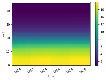
hovmoller diagram
[51]:
data = pf.get_data('../../DATA/LCORE/', 'temp', range(1948,1960), mesh, how="ori", compute=False )
Depth is None, 3d field will be returned
[52]:
vol = pf.hovm_data(data, mesh)
/Users/koldunovn/miniconda3/envs/pyfesom2/lib/python3.6/site-packages/dask/core.py:119: RuntimeWarning: invalid value encountered in true_divide
  return func(*args2)
[53]:
vol
[53]:
- time: 12
- nz1: 47
- 17.83 17.83 17.83 17.78 17.74 ... 0.9039 0.9398 0.9582 0.9941 nan
array([[17.82867066, 17.82899408, 17.82830539, 17.77710279, 17.73962606, 17.51843251, 17.11440206, 16.62482257, 16.18429902, 15.79307494, 15.41684823, 14.95335855, 14.31458113, 13.53615422, 12.70038638, 11.77183867, 10.79966389, 9.86239749, 8.9210438 , 7.97359661, 7.06789966, 6.24512426, 5.5062616 , 4.83223099, 4.25496992, 3.76676026, 3.37356564, 3.0199697 , 2.70289681, 2.39801439, 2.14765227, 1.95454626, 1.76355569, 1.61862895, 1.48711548, 1.37282054, 1.25944802, 1.15460584, 1.05162864, 0.97678949, 0.92469483, 0.90669904, 0.90098154, 0.94119623, 0.94740949, 0.96301914, nan], [17.73475652, 17.73486519, 17.73384975, 17.68291504, 17.63187864, 17.39332267, 16.98418657, 16.49846892, 16.08023646, 15.72736393, 15.39877952, 14.99272245, 14.42796166, 13.72603949, 12.93280937, 12.01163443, 10.9876912 , 9.97246293, 8.98037597, 7.99944048, 7.07056 , 6.23295111, 5.48934689, 4.82049205, 4.24781292, 3.76392545, 3.37203101, 3.02117141, 2.70391906, 2.39826537, 2.14887462, 1.95357655, 1.76466653, 1.61916447, 1.48946295, 1.37518082, 1.26338023, 1.15674513, 1.0535603 , 0.97565714, 0.92590966, 0.90528703, 0.90194199, 0.94034505, 0.94995893, 0.96895576, nan], [17.73921837, 17.7393508 , 17.73838334, 17.6848399 , 17.63239094, 17.39945577, 16.99708293, 16.5133969 , 16.09523171, 15.75634822, 15.44878557, 15.0725782 , 14.54728865, 13.88596701, 13.12535011, 12.22331532, 11.16005276, 10.0786899 , 9.03626735, 8.03002852, 7.08286587, 6.23324713, 5.48313917, 4.81481557, 4.24298249, 3.76060866, 3.36842279, 3.01960961, 2.70223098, 2.39754052, 2.14952375, 1.95255562, 1.76523577, 1.61958421, 1.49144169, 1.37711412, 1.26628628, 1.15890573, 1.05607538, 0.97645997, 0.92696678, 0.90470082, 0.90184984, 0.93980626, 0.95093437, 0.97341359, nan], [17.88621537, 17.88640514, 17.88557151, 17.84031306, 17.80871682, 17.59833276, 17.21051627, 16.72177866, 16.28851737, 15.92934665, 15.60316602, 15.20533965, 14.64469893, 13.94038784, 13.1430013 , 12.23456305, 11.18222546, 10.10785804, 9.05340607, 8.04015998, 7.0855793 , 6.22768621, 5.47329713, 4.80688168, 4.23639664, 3.75496522, 3.36344619, 3.01693424, 2.69996599, 2.39670498, 2.14946598, 1.95151919, 1.76580249, 1.62014467, 1.49312407, 1.37869968, 1.26836757, 1.16056564, 1.05827224, 0.97782071, 0.92821474, 0.90470258, 0.90186011, 0.93970678, 0.95178831, 0.97691568, nan], [17.94804789, 17.94821695, 17.94731012, 17.90553027, 17.88151105, 17.66518202, 17.25744373, 16.76310972, 16.34494901, 15.99987287, 15.67824801, 15.27776873, 14.70982653, 13.9904513 , 13.18015734, 12.24982478, 11.21302377, 10.1497885 , 9.08409091, 8.05356899, 7.0906565 , 6.22384698, 5.46430612, 4.80003496, 4.23118489, 3.75075767, 3.35979354, 3.01517326, 2.69887831, 2.39680604, 2.14996768, 1.95108626, 1.76666938, 1.62112833, 1.49493804, 1.38028997, 1.27007207, 1.16193499, 1.05986211, 0.97928911, 0.92949942, 0.90474364, 0.90178832, 0.93960585, 0.95265539, 0.98017565, nan], [17.98020813, 17.98041392, 17.97959895, 17.94007115, 17.9218282 , 17.72016501, 17.33119164, 16.8451182 , 16.42046036, 16.06686669, 15.7406817 , 15.3350055 , 14.76007409, 14.02881878, 13.20021407, 12.25702366, 11.21884605, 10.16166175, 9.09717184, 8.0656539 , 7.10103549, 6.22650021, 5.46141093, 4.79717423, 4.22901133, 3.74846627, 3.35685767, 3.01340449, 2.69770741, 2.39681475, 2.15047285, 1.95078017, 1.76740484, 1.62201961, 1.49664808, 1.3819823 , 1.27180641, 1.16342235, 1.06156209, 0.9809493 , 0.93075556, 0.90500647, 0.90180417, 0.93938971, 0.95354626, 0.98300487, nan], [17.81700055, 17.81723712, 17.81646659, 17.77524509, 17.74709348, 17.5441173 , 17.17083839, 16.716616 , 16.32902302, 16.00991394, 15.70910089, 15.33009956, 14.78848427, 14.09645326, 13.28894439, 12.33923547, 11.2722969 , 10.20041452, 9.12290561, 8.07850693, 7.10735441, 6.22817899, 5.46013291, 4.79600704, 4.22833755, 3.74711363, 3.35495639, 3.01212205, 2.69616257, 2.39633488, 2.15056899, 1.95032189, 1.76798281, 1.62303796, 1.49833512, 1.38383844, 1.27380738, 1.16514421, 1.06344823, 0.98283734, 0.93227749, 0.9056456 , 0.90196429, 0.93930413, 0.95435616, 0.98571882, nan], [17.77264178, 17.77284973, 17.7720491 , 17.73207292, 17.70339659, 17.49269354, 17.10767007, 16.63978747, 16.2375368 , 15.9083826 , 15.61008534, 15.24325165, 14.72852088, 14.07941298, 13.32355576, 12.41101383, 11.33446863, 10.2443172 , 9.15692751, 8.10217507, 7.12067826, 6.23265269, 5.4593405 , 4.79477147, 4.22756881, 3.74594522, 3.35259859, 3.01000923, 2.69418282, 2.39595089, 2.15068255, 1.9499168 , 1.76868326, 1.62393723, 1.49976045, 1.3857706 , 1.27599393, 1.16713994, 1.06559968, 0.9848428 , 0.933751 , 0.9062357 , 0.90214751, 0.93913647, 0.95516444, 0.98778081, nan], [17.77650489, 17.77671361, 17.77591237, 17.73790969, 17.71996732, 17.5202119 , 17.14954214, 16.68159024, 16.27418751, 15.93766541, 15.62882855, 15.25449312, 14.74072066, 14.10101766, 13.35970872, 12.46449811, 11.38095388, 10.26649725, 9.17926375, 8.12007785, 7.12909037, 6.23164264, 5.45483127, 4.79159874, 4.22632838, 3.74453926, 3.35005071, 3.00750899, 2.69193433, 2.3953069 , 2.15072555, 1.94959931, 1.76921663, 1.62475907, 1.50120936, 1.38753959, 1.27793629, 1.1689311 , 1.06744083, 0.98640774, 0.934891 , 0.90686216, 0.90238201, 0.93916167, 0.95589467, 0.98957784, nan], [17.97030038, 17.97051451, 17.96973818, 17.93227626, 17.91355965, 17.7152704 , 17.3367794 , 16.85407248, 16.43030652, 16.07616572, 15.74989054, 15.35284839, 14.79832066, 14.11197336, 13.33156821, 12.4088892 , 11.33992313, 10.25883171, 9.17999601, 8.12902007, 7.13773608, 6.23508854, 5.45258315, 4.78757358, 4.22278403, 3.74131102, 3.34639434, 3.00435681, 2.68951812, 2.39481252, 2.15087429, 1.94942709, 1.76993739, 1.62575438, 1.50283456, 1.38951942, 1.2802356 , 1.17116792, 1.06952085, 0.98806235, 0.93626863, 0.90760782, 0.90280887, 0.93942046, 0.95671303, 0.9911883 , nan], [17.9983345 , 17.99858823, 17.9978591 , 17.96650572, 17.96019132, 17.7700483 , 17.38810447, 16.90013982, 16.4718399 , 16.11846285, 15.78941497, 15.37866242, 14.79768373, 14.07281178, 13.26711814, 12.34486694, 11.31667846, 10.26037583, 9.19154301, 8.13995939, 7.14455769, 6.23834375, 5.45135764, 4.78536988, 4.22146454, 3.73957368, 3.34327001, 3.00132841, 2.68712085, 2.39405512, 2.15072265, 1.94915095, 1.77053371, 1.62671713, 1.50448664, 1.39166527, 1.28280143, 1.17379171, 1.07190868, 0.99030111, 0.93812547, 0.90853936, 0.90328807, 0.93947428, 0.95748658, 0.99280917, nan], [17.95737682, 17.95762813, 17.95690359, 17.92355643, 17.9067346 , 17.70916449, 17.33055523, 16.85877125, 16.45033109, 16.10868819, 15.78725508, 15.3873497 , 14.82268441, 14.11157839, 13.29899915, 12.35473266, 11.31549487, 10.26777632, 9.20339599, 8.15259462, 7.15346612, 6.24367958, 5.45382589, 4.78634935, 4.22104906, 3.73779901, 3.33989755, 2.99799427, 2.68446384, 2.39288878, 2.15037775, 1.94876839, 1.77117064, 1.6279751 , 1.50642526, 1.39413743, 1.28557613, 1.17666221, 1.07469848, 0.99292138, 0.94008829, 0.9096905 , 0.90388928, 0.93978891, 0.95822025, 0.99407875, nan]]) - time(time)datetime64[ns]1948-12-30T23:15:00 ... 1959-12-31T23:15:00
- long_name :
- time
array(['1948-12-30T23:15:00.000000000', '1949-12-31T23:15:00.000000000',
       '1950-12-31T23:15:00.000000000', '1951-12-31T23:15:00.000000000',
       '1952-12-30T23:15:00.000000000', '1953-12-31T23:15:00.000000000',
       '1954-12-31T23:15:00.000000000', '1955-12-31T23:15:00.000000000',
       '1956-12-30T23:15:00.000000000', '1957-12-31T23:15:00.000000000',
       '1958-12-31T23:15:00.000000000', '1959-12-31T23:15:00.000000000'],
      dtype='datetime64[ns]')
[54]:
vol.T.plot()
[54]:
<matplotlib.collections.QuadMesh at 0x12b24d7b8>
Volume weighted means
[55]:
temperature_0_500 = pf.volmean_data(data, mesh, [0, 500])
Upper depth: 0.0, Lower depth: -490.0
[56]:
temperature_0_500
[56]:
- time: 12
- dask.array<chunksize=(1,), meta=np.ndarray>
Array Chunk Bytes 96 B 8 B Shape (12,) (1,) Count 2100 Tasks 12 Chunks Type float64 numpy.ndarray - time(time)datetime64[ns]1948-12-30T23:15:00 ... 1959-12-31T23:15:00
- long_name :
- time
array(['1948-12-30T23:15:00.000000000', '1949-12-31T23:15:00.000000000',
       '1950-12-31T23:15:00.000000000', '1951-12-31T23:15:00.000000000',
       '1952-12-30T23:15:00.000000000', '1953-12-31T23:15:00.000000000',
       '1954-12-31T23:15:00.000000000', '1955-12-31T23:15:00.000000000',
       '1956-12-30T23:15:00.000000000', '1957-12-31T23:15:00.000000000',
       '1958-12-31T23:15:00.000000000', '1959-12-31T23:15:00.000000000'],
      dtype='datetime64[ns]')
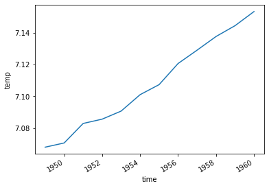
[57]:
temperature_500 = pf.volmean_data(data, mesh, [500, 500])
Upper depth: -490.0, Lower depth: -490.0
[58]:
temperature_500.plot()
[58]:
[<matplotlib.lines.Line2D at 0x12c88b278>]
Low level functions
Getting the data
Main function get_data from load_mesh_data.py:
get_data(
    result_path,
    variable,
    years,
    mesh,
    runid="fesom",
    records=-1,
    depth=None,
    how="mean",
    ncfile=None,
    compute=True,
    continuous=False,
    **kwargs
    )
Mainly wraper around xarray.open_mfdataset, plus some default aggregation operations.
Interpolation
Main function is fesom2regular from regriding.py:
fesom2regular(
    data,
    mesh,
    lons,                 # regular 2d
    lats,                 # regular 2d
    distances_path=None,  # we store interpolation weights
    inds_path=None,       # we store interpolation weights
    qhull_path=None,      # we store interpolation weights
    how="nn",             # several types of interpolation, KDTree based and from scipy
    k=5,
    radius_of_influence=100000, # can be dificult for meshes with very different resolutions
    n_jobs=2,             # can be parallel
    dumpfile=True,        # we store interpolation weights
    basepath=None,        # we store interpolation weights
):
Variables on elements are first interpolated to nodes and then to regular grid for plotting:
tonodes
tonodes3d
Selection
By points (e.g., transect)
We initially work with some collection of points. Usually it’s a straight line, generated by transect_get_lonlat function from start and end point coordinates, as well as the number of points in between. However it can be just collection of any points.
Select model mesh nodes that are closest to the “observational” points. Use the
tunnel_fast1dfunction. This is a serial process (one point at a time), and for large meshes is slow. Can be optimised. The result isnodes[number_of_nodes]variable with boolian values, that are true, if the node is selected (closest to “observations”).Select nodes from FESOM2 3D data (
data3D[number_of_nodes, number_of_levels]) by doingtransect_data = data3d[nodes, :]Mask nodes that are too far away (
max_distance) from original points (e.g. points are on land).
By bounding box (e.g., Area)
We just select nodes by lon/lat bounds, and get them from the data:
[59]:
box=[-160, -147, 71, 73]
left, right, down, up = box
mask_al = ((mesh.x2 >= left) &
           (mesh.x2 <= right) &
           (mesh.y2 >= down) &
           (mesh.y2 <= up))
[60]:
temp.shape
[60]:
(126858, 47)
[61]:
temp[mask_al,:].shape
[61]:
(182, 47)
Weighted area mean
We need areas associated with each node at each level. For this additional meshdiag file is loaded. It is generated before the first timestep of the model cold start, and usually available in the mesh path.
[62]:
meshdiag = pf.get_meshdiag(mesh)
We only need nod_area from this file:
[63]:
nod_area = np.ma.masked_equal(meshdiag.nod_area.values, 0)
[64]:
temp_by_area = ((np.ma.masked_equal(temp[mask_al,:],0) * nod_area[:-1,:].T[mask_al]).mean(axis=0))
[65]:
temp_weighted = temp_by_area/nod_area[:-1,:].T[mask_al].mean(axis=0)
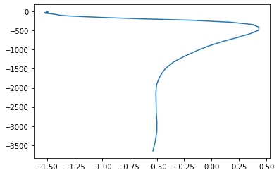
[66]:
plt.plot(temp_weighted, mesh.zlev[:-1],)
[66]:
[<matplotlib.lines.Line2D at 0x12dd7deb8>]
Vertical integral
[67]:
(temp_weighted[:]*np.diff(mesh.zlev[:]*-1)).sum()
[67]:
-1422.1065271404095
Weighted mean
[68]:
((temp_weighted[:]*np.diff(mesh.zlev[:]*-1)).sum())/np.diff(mesh.zlev[:]*-1).sum()
[68]:
-0.22753704434246552
[ ]: