This page was generated from notebooks/compute_MOC.ipynb. Interactive online version: .

MOC computation

If you would like to try to repeat examples from this notebook, you can download FESOM2 data and mesh. The data are quite heavy, about 15 Gb.

Link: https://swiftbrowser.dkrz.de/public/dkrz_c719fbc3-98ea-446c-8e01-356dac22ed90/PYFESOM2/

You have to download both archives (LCORE.tar and LCORE_MESH.tar) and extract them.

Alternative would be to use very light weight mesh that comes with pyfesom2 in the tests/data/pi-grid/ and example data on this mesh in tests/data/pi-results.

import pyfesom2 as pf
import matplotlib.cm as cm
import matplotlib.pylab as plt
import numpy as np

mesh = pf.load_mesh('/Users/koldunovn/PYHTON/DATA/LCORE_MESH/',
                    abg=[50, 15, -90])

/Users/koldunovn/PYHTON/DATA/LCORE_MESH/pickle_mesh_py3_fesom2
The usepickle == True)
The pickle file for FESOM2 exists.
The mesh will be loaded from /Users/koldunovn/PYHTON/DATA/LCORE_MESH/pickle_mesh_py3_fesom2

data = pf.get_data('../../DATA/LCORE/', 'w', range(1950,1959), mesh, how="mean", compute=True )

Depth is None, 3d field will be returned

data.shape

(126858, 48)

Minimum nessesary input is mesh and one 3D field of w.

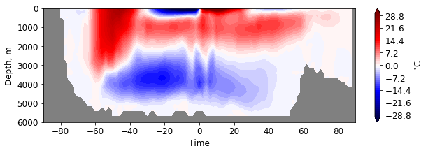
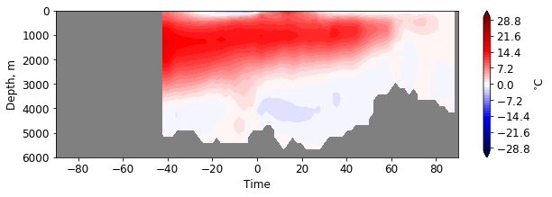
lats, moc = pf.xmoc_data(mesh, data)

You get latitides and the MOC values (global by default). They can be used to plot the MOC using hofm_plot function:

plt.figure(figsize=(10, 3))
pf.hofm_plot(mesh, moc, xvals=lats, maxdepth=7000, cmap=cm.seismic, levels = np.linspace(-30, 30, 51),
             facecolor='gray')

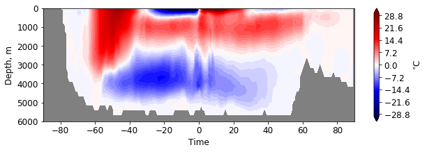
Increase the number of latitude bins:

lats, moc = pf.xmoc_data(mesh, data, nlats=200)

plt.figure(figsize=(10, 3))
pf.hofm_plot(mesh, moc, xvals=lats, maxdepth=7000, cmap=cm.seismic, levels = np.linspace(-30, 30, 51),
             facecolor='gray')

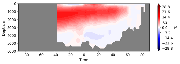
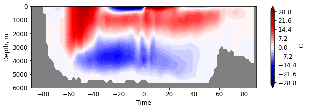
You can define the region for MOC computation.

lats, moc = pf.xmoc_data(mesh, data, mask="Atlantic_MOC")

plt.figure(figsize=(10, 3))
pf.hofm_plot(mesh, moc, xvals=lats, maxdepth=7000, cmap=cm.seismic, levels = np.linspace(-30, 30, 51),
             facecolor='gray')

Regions are listed in documentation of pf.get_mask. Currently they are:

Ocean Basins:
     "Atlantic_Basin"
     "Pacific_Basin"
     "Indian_Basin"
     "Arctic_Basin"
     "Southern_Ocean_Basin"
     "Mediterranean_Basin"
     "Global Ocean"
     "Global Ocean 65N to 65S"
     "Global Ocean 15S to 15N"
 MOC Basins:
     "Atlantic_MOC"
     "IndoPacific_MOC"
     "Pacific_MOC"
     "Indian_MOC"
 Nino Regions:
     "Nino 3.4"
     "Nino 3"
     "Nino 4"

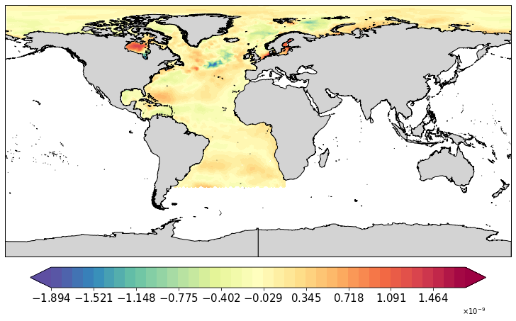
You can combine masks:

mask1 = pf.get_mask(mesh, "Atlantic_Basin")
mask2 = pf.get_mask(mesh, "Arctic_Basin")
mask3 = mask1|mask2

Check how the masked data looks like:

pf.plot(mesh, data[:,0]*mask3)

[<cartopy.mpl.geoaxes.GeoAxesSubplot at 0x11ed73ef0>]

You can then provide combined mask to xmoc_data:

lats, moc = pf.xmoc_data(mesh, data, mask=mask3)

plt.figure(figsize=(10, 3))
pf.hofm_plot(mesh, moc, xvals=lats, maxdepth=7000, cmap=cm.seismic, levels = np.linspace(-30, 30, 51),
             facecolor='gray')

If you work with large meshes, it makes sence to compute some data beforehand and provide them to the function:

meshdiag = pf.get_meshdiag(mesh)
el_area = meshdiag['elem_area'][:]
nlevels = meshdiag['nlevels'][:]-1
face_x, face_y = pf.compute_face_coords(mesh)
mask = pf.get_mask(mesh, 'Global Ocean')

lats, moc = pf.xmoc_data(mesh, data, mask = mask,
                el_area = el_area, nlevels=nlevels,
                face_x=face_x, face_y=face_y)

plt.figure(figsize=(10, 3))
pf.hofm_plot(mesh, moc, xvals=lats, maxdepth=7000, cmap=cm.seismic, levels = np.linspace(-30, 30, 51),
             facecolor='gray')

Compute AMOC at 26.5N

Open data as time series

data = pf.get_data('../../DATA/LCORE/', 'w', range(1950,1959), mesh, how="ori", compute=False )

Depth is None, 3d field will be returned

data

xarray.DataArray

'w'

• time: 9
• nod2: 126858
• nz: 48

• dask.array<chunksize=(1, 126858, 48), meta=np.ndarray>

  
  
  
  
    
  
      
   
   Array 
   Chunk 
    
    
  
      
   Bytes 
   219.21 MB 
   
   24.36 MB 
      
   Shape 
   (9, 126858, 48) 
   
   (1, 126858, 48) 
      
   Count 
   27 Tasks 
   9 Chunks 
      
   Type 
   float32 
   numpy.ndarray 
    
  
  
  
  
  
  
  

• Coordinates: (1)
  • time
    (time)
    datetime64[ns]
    1950-12-31T23:15:00 ... 1958-12-31T23:15:00

    long_name :

    time

    array(['1950-12-31T23:15:00.000000000', '1951-12-31T23:15:00.000000000',
           '1952-12-30T23:15:00.000000000', '1953-12-31T23:15:00.000000000',
           '1954-12-31T23:15:00.000000000', '1955-12-31T23:15:00.000000000',
           '1956-12-30T23:15:00.000000000', '1957-12-31T23:15:00.000000000',
           '1958-12-31T23:15:00.000000000'], dtype='datetime64[ns]')

• Attributes: (2)

  description :

  vertical velocity

  units :

  m/s

We have 9 time steps

data.shape

(9, 126858, 48)

Compute AMOC for each time step, increase the number of latitudes if you want to be preciselly at 26.5:

moc = []

for i in range(data.shape[0]):
    lats, moc_time = pf.xmoc_data(mesh, data[i,:,:], mask='Atlantic_MOC', nlats=361)
    moc.append(moc_time)

Find which index corresponds to 26.5

lats[233]

26.5

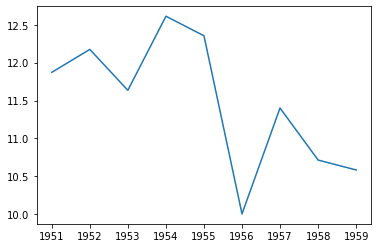
Compute maximum at this point for each time step:

amoc26 = []
for i in range(len(moc)):
    amoc26.append(moc[i][233,:].max())

amoc26

[11.871677395438851,
 12.17447911245645,
 11.634695012527837,
 12.611884810155964,
 12.354251356017224,
 10.003526012070289,
 11.40134476396998,
 10.713783333512506,
 10.583684577084185]

You can use time information from original dataset for plotting:

plt.plot(data.time, amoc26)

[<matplotlib.lines.Line2D at 0x11eb854a8>]