pfplot
Plots scalar from FESOM mesh interpolated on regular grid.
There is a lot in common with options from pfinterp, so we will refer to its documentation instead of repeating.
Basic usage
As a minimum you should provide path to the mesh, path to the file, path were the ouptut will be stored and variable name:
pfplot /path/to/mesh/ /path/to/datafolder/ temp
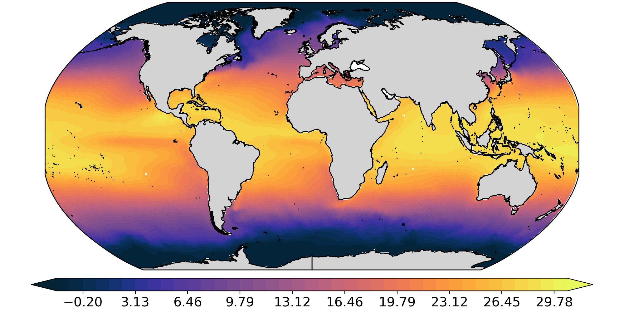
by default pfplot will search for the year 1948 and interpolate first time step from the depth 0 to 1 degree lon/lat regular grid and display it on the screen.
In the following we just going to replace paths by shell variables:
MESH=/path/to/mesh/
DATA=/path/to/datafolder/
to make examples more consise. It is also a good practice to setup such variables for yourself, so the commands are shorter.
You can get help with list of all available options by executing:
pfplot --help
Data selection and interpolation options
All interpolation and data selection options are identical to pfinterp. See respective sections on Time selection, Depth selection and Interpolation.
Plotting options
Projections
Plot ptojection is controlled by the -m option. At the moment only five projections are available:
Mercator (merc),
Plate Carree (pc),
North Polar Stereo (np),
South Polar Stereo (sp),
Robinson (rob).
Deafault is Robinson projection.
The map region is defined by the -b option, so in order to obtain usuall plot in North Polar Stereo projection, that covers region to the north of 60N
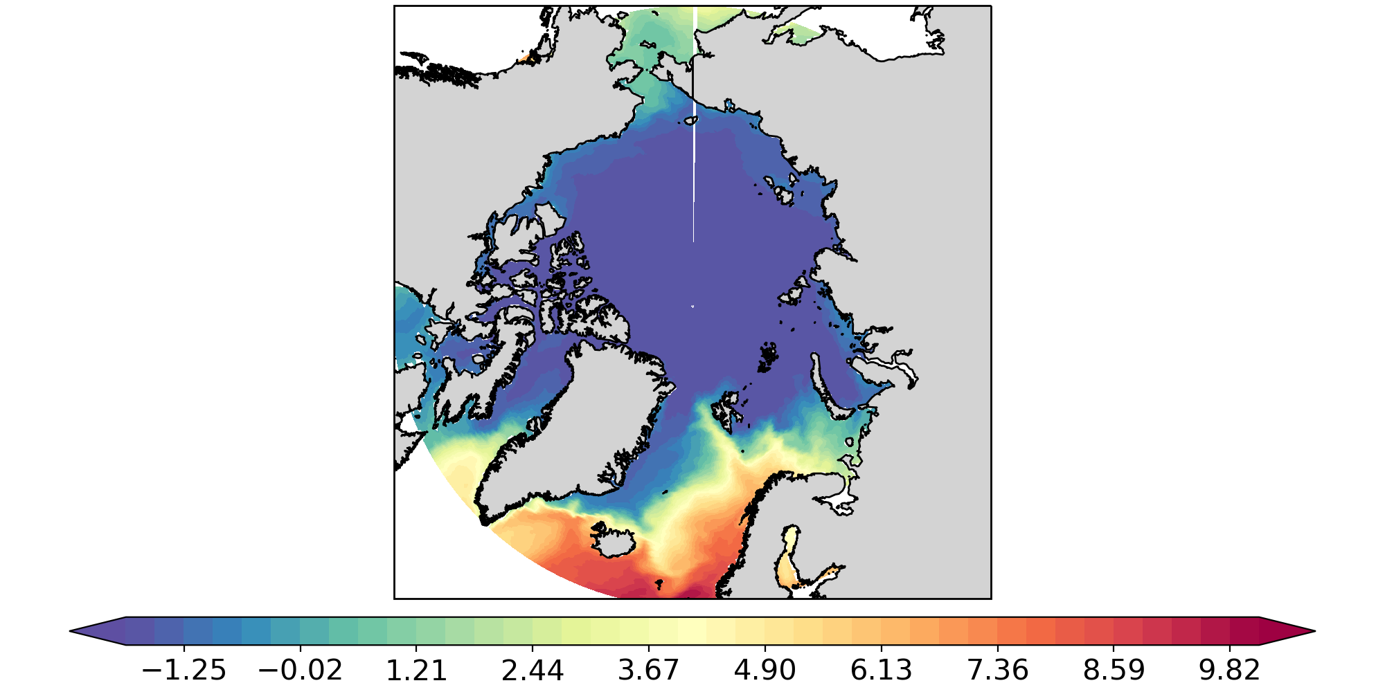
one should adjust the region:
pfplot $MESH $DATA temp -b -180 180 60 90 -m np
Colormaps
Colormaps are controlled by –cmap option. The default colormap is matplotlib’s Spectral_r. One can provide any colormap name from cmocean package or from the standard matplotlib set:
pfplot $MESH $DATA temp --cmap thermal
Levels
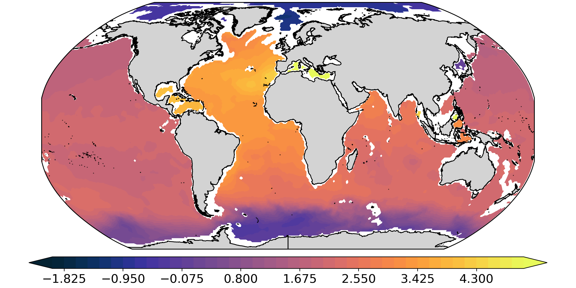
Levels fro the countour plot are controlled by -l opetion. One has to provide 3 values: minimum, maximum and the number of levels (they will be used for numpy linspace function). The following command will plot global map of temperature at 2000 m depth with thetmal colormap from cmocean and 41 level from -2 to 5:
pfplot $MESH $DATA temp --cmap thermal -d 2000 -l -2 5 41
Plot type
Two plot types are availabale: contourf (cf) and pcolormesh (pcm). They are controlled through –ptype option. In some cases pcm might be faster than cf, espetially when the field is not smooth and a lot of contour levels should be generated.